12 - Monstros e Misturas
Imports, loadings and functions
import numpy as np

from scipy import stats

import matplotlib.pyplot as plt
from matplotlib.gridspec import GridSpec

import pandas as pd

import networkx as nx
# from causalgraphicalmodels import CausalGraphicalModel

import arviz as az
# ArviZ ships with style sheets!
# https://python.arviz.org/en/stable/examples/styles.html#example-styles
az.style.use("arviz-darkgrid")

import xarray as xr

import stan
import nest_asyncio

plt.style.use('default')
plt.rcParams['axes.facecolor'] = 'lightgray'

# To DAG's
import daft
from causalgraphicalmodels import CausalGraphicalModel
# Add fonts to matplotlib to run xkcd

from matplotlib import font_manager

font_dirs = ["fonts/"]  # The path to the custom font file.
font_files = font_manager.findSystemFonts(fontpaths=font_dirs)

for font_file in font_files:
    font_manager.fontManager.addfont(font_file)
# To make plots like drawing
# plt.xkcd()
# To running the stan in jupyter notebook
nest_asyncio.apply()
# Utils functions

def logit(p):
    return np.log(p) - np.log(1 - p)

def inv_logit(p):
    return np.exp(p) / (1 + np.exp(p))
12.1 Over-dispersed counts
12.1.1 Beta-Binomial
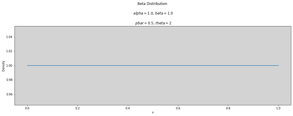
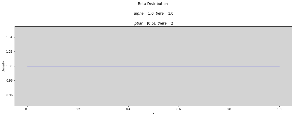
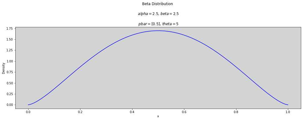
Beta distributuion:
another parametrization:
where: $\( \alpha = \bar{p} \theta \)$
R Code 12.1
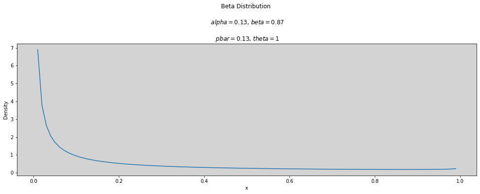
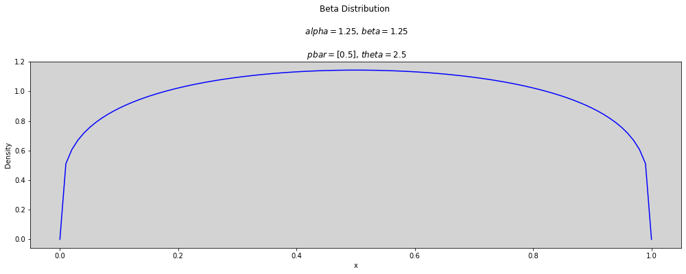
def plot_beta(p_bar, theta):
    alpha = p_bar * theta  # Alpha = p * theta
    beta = (1 - p_bar) * theta  # beta = (1-p) * theta

    x = np.linspace(0, 1, num=100)

    plt.figure(figsize=(17, 5))

    plt.plot(x, stats.beta.pdf(x, alpha, beta))

    plt.title(f'Beta Distribution \n\n $alpha={round(alpha, 3)}$, $beta={round(beta, 3)}$ \n\n $pbar={p_bar}$, $theta={theta}$')
    plt.ylabel('Density')
    plt.xlabel('x')
    plt.show()
p_bar = 0.5
theta = 2
plot_beta(p_bar, theta)
# -----
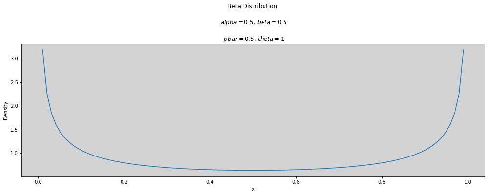
p_bar = 0.5
theta = 1
plot_beta(p_bar, theta)
# -----
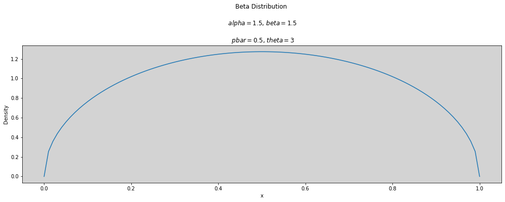
p_bar = 0.5
theta = 3
plot_beta(p_bar, theta)
# -----
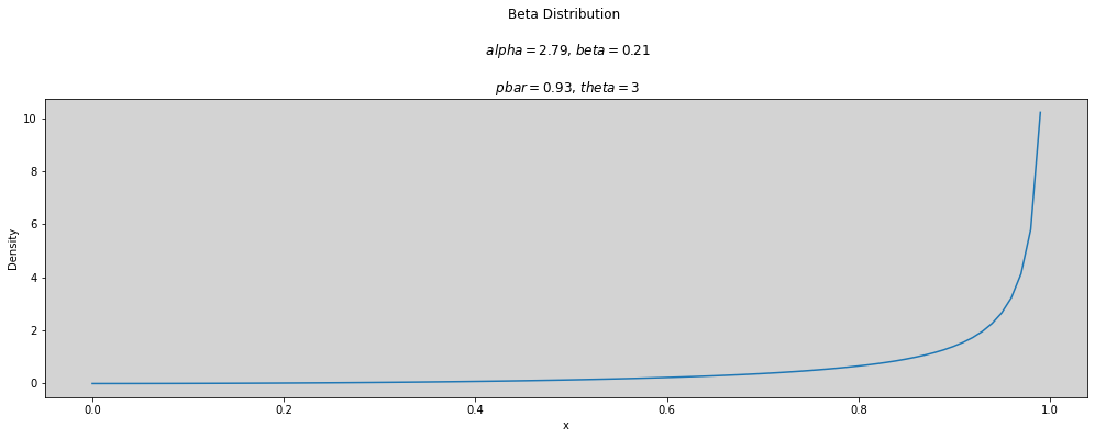
p_bar = 0.93 # 0 < p < 1
theta = 3
plot_beta(p_bar, theta)
# -----
p_bar = 0.13 # 0 < p < 1
theta = 1
plot_beta(p_bar, theta)
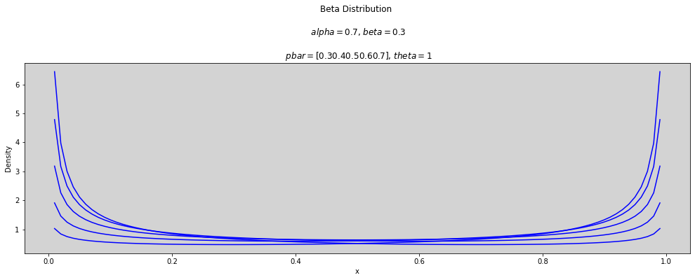
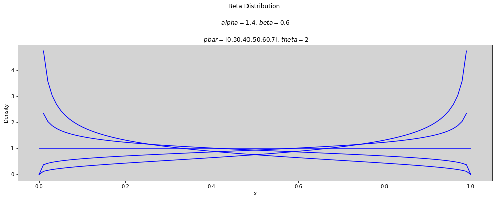
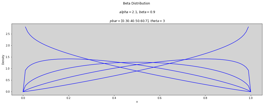
p_bar = np.arange(0.3, 0.8, 0.1)  # array([0.3, ..., 0.7])
theta = [1, 2, 3]

x = np.linspace(0, 1, num=100)


for t in theta:
    plt.figure(figsize=(17, 5))
    for p in p_bar:
        alpha = p * t
        beta = (1 - p) * t

        plt.plot(x, stats.beta.pdf(x, alpha, beta), c='blue')

        plt.title(f'Beta Distribution \n\n $alpha={round(alpha, 3)}$, $beta={round(beta, 3)}$ \n\n $pbar={p_bar}$, $theta={round(t, 3)}$')
        plt.ylabel('Density')
        plt.xlabel('x')
    plt.show()
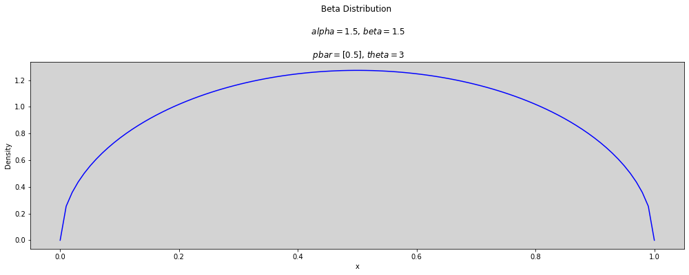
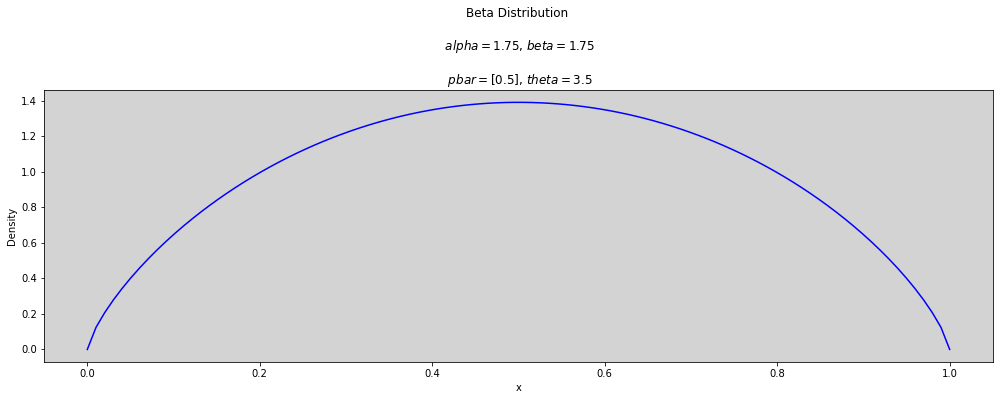
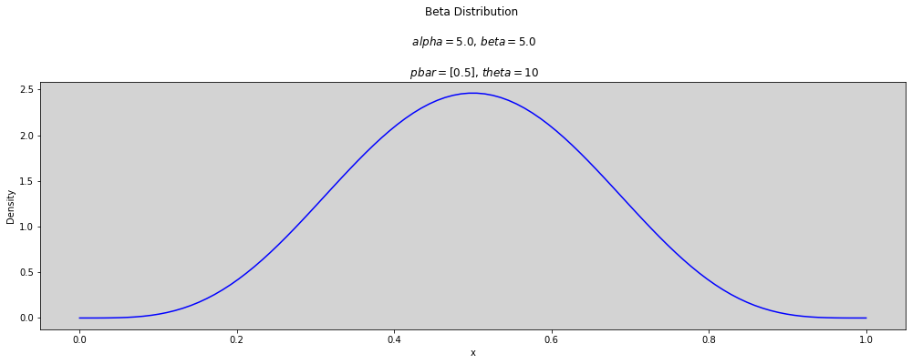
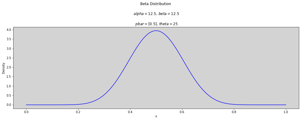
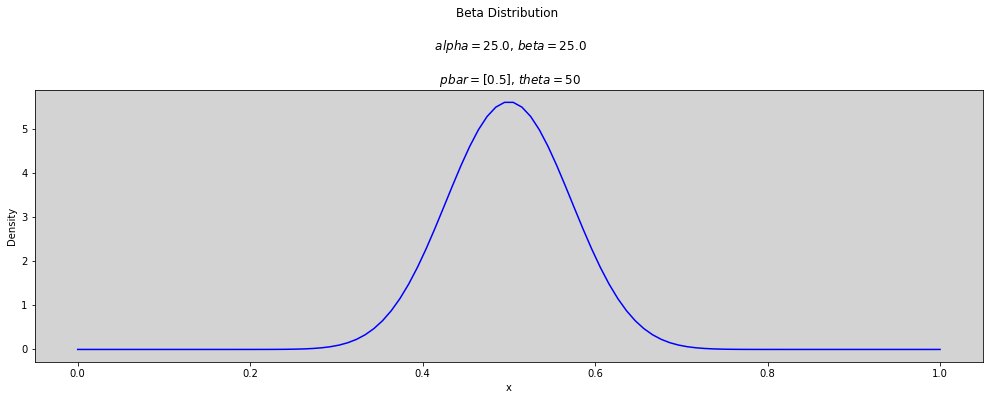
p_bar = [0.5]
theta = [2, 2.5, 3, 3.5, 5, 10, 25, 50]

x = np.linspace(0, 1, num=100)


for t in theta:
    plt.figure(figsize=(17, 5))
    for p in p_bar:
        alpha = p * t
        beta = (1 - p) * t

        plt.plot(x, stats.beta.pdf(x, alpha, beta), c='blue')

        plt.title(f'Beta Distribution \n\n $alpha={round(alpha, 3)}$, $beta={round(beta, 3)}$ \n\n $pbar={p_bar}$, $theta={round(t, 3)}$')
        plt.ylabel('Density')
        plt.xlabel('x')
    plt.show()
R Code 12.2
The Beta-binomial model
Where:
\(A := \)
admit\(N := \)
applicantions\(GID[i] := \)
gidis gender index, \(1\) to male \(2\) to female
The BetaBinomial distribution in Stan has the parameters like most common Beta distribuiton. Then, the model above will be rewriter like:
Where:
\(A := \)
admit\(N := \)
applicantions\(GID[i] := \)
gidis gender index, \(1\) to male \(2\) to female\(\bar{p}_i := \) An average probability to gender type \(i\)
\(\theta := \) Shape of parameter, describe how spread out the distribution is.
Remember that binomial model for UCBadmit data, defined in 11.29, was written as follow:
df = pd.read_csv('./data/UCBadmit.csv', sep=';')
df['gid'] = [ 1 if gender == 'male' else 2 for gender in df['applicant.gender'] ]
df
| dept | applicant.gender | admit | reject | applications | gid | |
|---|---|---|---|---|---|---|
| 1 | A | male | 512 | 313 | 825 | 1 |
| 2 | A | female | 89 | 19 | 108 | 2 |
| 3 | B | male | 353 | 207 | 560 | 1 |
| 4 | B | female | 17 | 8 | 25 | 2 |
| 5 | C | male | 120 | 205 | 325 | 1 |
| 6 | C | female | 202 | 391 | 593 | 2 |
| 7 | D | male | 138 | 279 | 417 | 1 |
| 8 | D | female | 131 | 244 | 375 | 2 |
| 9 | E | male | 53 | 138 | 191 | 1 |
| 10 | E | female | 94 | 299 | 393 | 2 |
| 11 | F | male | 22 | 351 | 373 | 1 |
| 12 | F | female | 24 | 317 | 341 | 2 |
model = """
    functions {
        vector alpha_cast(vector pbar, real theta){
            return pbar * theta;
        }

        vector beta_cast(vector pbar, real theta){
            return (1-pbar) * theta;
        }
    }

    data {
        int N;
        int qty_gid;
        array[N] int admit;
        array[N] int applications;
        array[N] int gid;
    }

    parameters {
        vector[qty_gid] a;
        real<lower=0> phi;
    }

    transformed parameters {
        real<lower=2> theta;  // Need declared here to transform the parameter
        theta = phi + 2;
    }

    model {
        vector[N] pbar;

        a ~ normal(0, 1.5);
        phi ~ exponential(1);

        for (i in 1:N){
            pbar[i] = a[ gid[i] ];
            pbar[i] = inv_logit(pbar[i]);
        }

        admit ~ beta_binomial(applications, alpha_cast(pbar, theta), beta_cast(pbar, theta) );
    }

    generated quantities {
        real da;
        da = a[1] - a[2];
    }

"""

data_list = df[['applications', 'admit', 'gid']].to_dict('list')
data_list['N'] = len(df.admit)
data_list['qty_gid'] = len(df.gid.unique())
data_list

posteriori = stan.build(model, data=data_list)
samples = posteriori.sample(num_chains=4, num_samples=1000)
model_12_1 = az.from_pystan(
    posterior=samples,
    posterior_model=posteriori,
    observed_data=list(data_list.keys()),
    dims={
        'a': ['gender'],
    }
)
R Code 12.3
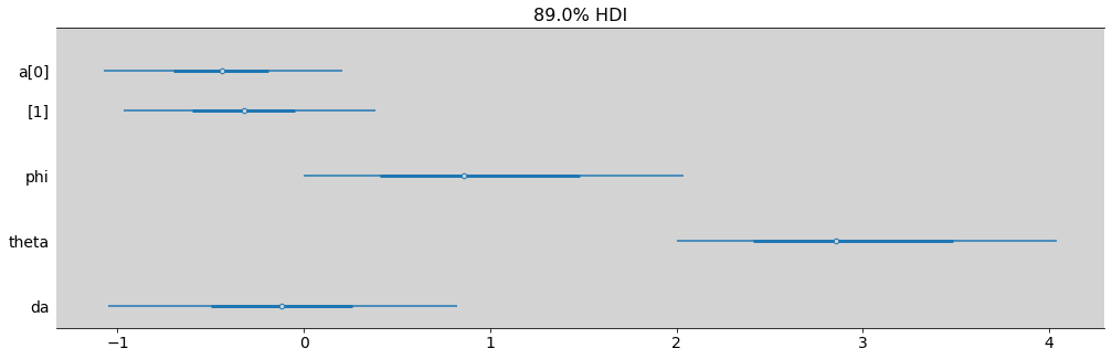
az.summary(model_12_1, hdi_prob=0.89)
| mean | sd | hdi_5.5% | hdi_94.5% | mcse_mean | mcse_sd | ess_bulk | ess_tail | r_hat | |
|---|---|---|---|---|---|---|---|---|---|
| a[0] | -0.444 | 0.401 | -1.071 | 0.206 | 0.007 | 0.006 | 3017.0 | 2336.0 | 1.0 |
| a[1] | -0.326 | 0.422 | -0.966 | 0.384 | 0.008 | 0.007 | 3088.0 | 2596.0 | 1.0 |
| phi | 1.026 | 0.794 | 0.002 | 2.040 | 0.014 | 0.010 | 2232.0 | 1312.0 | 1.0 |
| theta | 3.026 | 0.794 | 2.002 | 4.040 | 0.014 | 0.010 | 2232.0 | 1312.0 | 1.0 |
| da | -0.117 | 0.584 | -1.050 | 0.822 | 0.011 | 0.010 | 2961.0 | 2170.0 | 1.0 |
az.plot_forest(model_12_1, combined=True, figsize=(17, 5), hdi_prob=0.89)
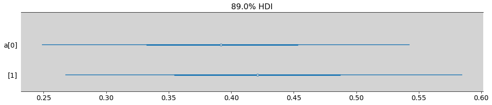
az.plot_forest(model_12_1, var_names=['a'], combined=True, figsize=(17, 3), hdi_prob=0.89, transform=inv_logit)
plt.show()
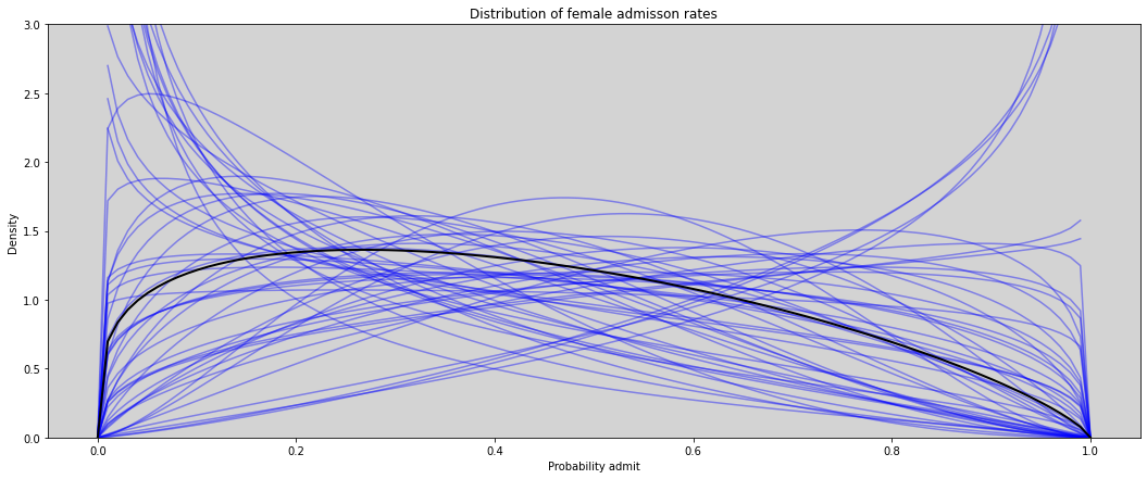
R Code 12.4
gid = 2  # female

p = inv_logit(model_12_1.posterior.a.sel(gender=1))
theta = model_12_1.posterior.theta

# Plot beta distribution posterior

alpha = p * theta  # Alpha = p * theta
beta = (1 - p) * theta  # beta = (1-p) * theta

plt.figure(figsize=(18, 7))

for i in range(50):
    plt.plot(x, stats.beta.pdf(x, alpha.values.flatten()[i], beta.values.flatten()[i]), c='blue', alpha=0.4)

plt.plot(x, stats.beta.pdf(x, alpha.values.mean(), beta.values.mean()), c='black', lw=2)

plt.ylim(0, 3)

plt.title(f'Distribution of female admisson rates')
plt.ylabel('Density')
plt.xlabel('Probability admit')

plt.show()
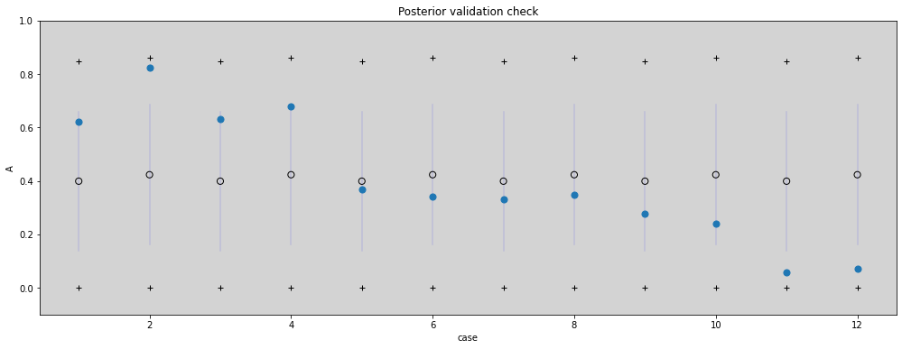
R Code 12.5
p_m = inv_logit(model_12_1.posterior.a.sel(gender=0).values.flatten())  # Male
p_f = inv_logit(model_12_1.posterior.a.sel(gender=1).values.flatten())  # Female

theta = model_12_1.posterior.theta.values.flatten()

# Calculation of alpha and beta to Beta distribution
alpha_m = p_m*theta
beta_m = (1 - p_m)*theta

alpha_f = p_f*theta
beta_f = (1 - p_f)*theta

p_bar_m = np.random.beta(alpha_m, beta_m)
p_bar_f = np.random.beta(alpha_f, beta_f)

hdi_m = az.hdi(p_bar_m)
hdi_f = az.hdi(p_bar_f)

mean_m = np.mean(p_bar_m)
mean_f = np.mean(p_bar_f)
for i in range(10, 2):
    print(i)
plt.figure(figsize=(17, 6))

for i in range(1, len(df), 2):
    # Male
    plt.plot([i, i], [mean_m - np.std(p_bar_m), np.std(p_bar_m) + mean_m ], c='blue', alpha=0.1)
    plt.plot(i, hdi_m[0], '+', c='k')
    plt.plot(i, hdi_m[1], '+', c='k')

    i = i + 1

    # Female
    plt.plot([i, i], [mean_f - np.std(p_bar_f), np.std(p_bar_f) + mean_f ], c='blue', alpha=0.1)
    plt.plot(i, hdi_f[0], '+', c='k')
    plt.plot(i, hdi_f[1], '+', c='k')

plt.scatter(range(1, len(df)+1), df.admit.values/df.applications.values, s=50, zorder=13)
plt.scatter(range(1, len(df)+1), [ mean_m if i == 1 else mean_f for i in df.gid ], facecolors='none', edgecolors='black', s=50, zorder=13)

plt.title('Posterior validation check')
plt.xlabel('case')
plt.ylabel('A')

plt.ylim(-0.1, 1)
plt.show()
12.1.2 Negative-binomial or Gamma-Poisson
The \(\lambda\) parameter can be treated like the rate of an ordinary Poisson.
The \(\phi\) parameter must be positive and controls the variance.
The variance of the Gamma-Poisson is \(\lambda + \lambda^2 \over \phi\).
The larges \(\phi\) values mean is similar to a pure Poisson process.
R Code 12.6 - TODO
df = pd.read_csv('./data/Kline.csv', sep=';')
df['P'] = ( np.log(df.population) - np.mean(np.log(df.population)) ) / np.std(np.log(df.population))
df['contact_id'] = [2 if contact_i == 'high' else 1 for contact_i in df.contact ]
df
| culture | population | contact | total_tools | mean_TU | P | contact_id | |
|---|---|---|---|---|---|---|---|
| 0 | Malekula | 1100 | low | 13 | 3.2 | -1.361332 | 1 |
| 1 | Tikopia | 1500 | low | 22 | 4.7 | -1.147433 | 1 |
| 2 | Santa Cruz | 3600 | low | 24 | 4.0 | -0.543664 | 1 |
| 3 | Yap | 4791 | high | 43 | 5.0 | -0.346558 | 2 |
| 4 | Lau Fiji | 7400 | high | 33 | 5.0 | -0.046737 | 2 |
| 5 | Trobriand | 8000 | high | 19 | 4.0 | 0.007029 | 2 |
| 6 | Chuuk | 9200 | high | 40 | 3.8 | 0.103416 | 2 |
| 7 | Manus | 13000 | low | 28 | 6.6 | 0.341861 | 1 |
| 8 | Tonga | 17500 | high | 55 | 5.4 | 0.546861 | 2 |
| 9 | Hawaii | 275000 | low | 71 | 6.6 | 2.446558 | 1 |
model = """
    data {
        int N;
        int qty_contact;
        array[N] int total_tools;
        array[N] int population;
        array[N] int contact_id;
    }

    parameters {
        array real[qty_contact] a;
        array real[qty_contact] b;
    }

    model {
        vector[N] lambda;
        real phi;

        phi ~ exponential(1);

        total_tools ~ neg_binomial(alpha, beta);
    }
"""
12.2 Zero-Inflated outcomes
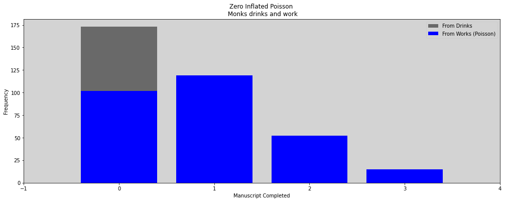
12.2.1 Example: Zero-inflated Poisson
Coin flip, with probability \(p\) that show “cask of wine” on one side and a quill on the other.
When monks is drinks, then none manuscript was be complete.
When hes are working, the manuscript are complete like the Poisson distribution on the average rate \(\lambda\).
The likelihood of a zero value \(y\) is:
In above is just a math form to:
The probability of observing a zero is the probability that the monks did drink OR (\(+\)) the probability that the monks worked AND (\(\times\)) failed to finish anything.
And the likelihood of a non-zero value \(y\) is:
The probability that monks working, \(1-p\), and finish \(y\) manuscripts. Since the drinking monks, \(p\), never finish any manuscript.
The ZIPoisson, with parameters \(p\) (probability of a zeros) and \(\lambda\) (rate mean of Poisson) to describe the shape.
The zero-inflated Poisson regression is that form:
R Code 12.7
prob_drink = 0.2  # 20% of days
rate_work = 1  # average 1 manuscript per day

# Samples one year of production
N = 365

# Simulate days monks drink
drink = np.random.binomial(n=1, p=prob_drink, size=N)
print('Drink day == 1')
print(drink)

# Simulate manuscript completed
y = (1 - drink) * np.random.poisson(lam=rate_work, size=N)
print('\n Work day')
print(y)
Drink day == 1
[0 0 0 0 1 0 0 0 0 0 1 0 0 0 0 1 0 0 1 0 0 0 1 0 0 0 0 0 1 0 0 0 0 0 1 0 1
 0 0 0 0 0 0 0 0 0 0 0 0 0 0 0 0 0 1 0 0 0 0 1 0 0 0 0 0 0 1 0 0 1 0 0 0 0
 0 1 0 0 0 0 0 0 1 0 0 1 1 1 0 0 0 0 0 0 0 1 0 0 1 0 1 0 1 0 0 0 1 1 0 1 0
 0 1 1 0 0 0 1 0 0 0 0 0 0 0 0 0 1 1 0 0 0 1 0 1 0 0 0 0 0 0 0 0 1 0 0 0 0
 0 0 0 0 0 0 0 0 0 0 0 0 0 0 0 1 0 0 1 1 0 0 0 1 0 0 0 0 0 1 0 0 0 0 0 0 0
 0 0 1 0 0 0 0 0 1 0 0 0 0 1 0 0 0 0 0 0 0 0 1 0 0 0 0 0 1 0 0 0 0 1 0 0 0
 0 1 0 0 1 0 0 0 1 0 0 0 0 1 0 0 0 0 0 0 0 0 1 0 0 0 0 1 0 0 0 0 0 1 0 0 0
 0 0 1 0 0 0 0 1 0 0 0 0 0 0 0 0 1 0 0 0 0 0 0 1 0 0 0 0 0 0 0 0 0 0 1 0 0
 0 0 0 0 0 0 0 0 0 1 0 0 0 0 1 0 1 1 0 0 0 1 0 0 1 0 0 0 0 0 0 1 0 0 1 1 0
 0 0 0 0 0 0 0 0 0 0 0 0 0 0 0 1 0 0 1 0 0 1 0 0 0 0 1 0 1 1 1 0]

 Work day
[1 2 0 0 0 0 0 1 1 1 0 0 0 3 4 0 1 1 0 0 2 1 0 1 2 2 1 0 0 1 1 2 0 3 0 2 0
 2 1 0 2 0 1 0 1 1 1 3 1 2 2 1 1 1 0 2 0 1 1 0 1 1 0 1 0 0 0 1 2 0 0 0 0 1
 0 0 0 0 1 0 1 0 0 0 0 0 0 0 3 0 0 0 3 0 1 0 1 1 0 1 0 1 0 0 2 1 0 0 1 0 3
 0 0 0 2 4 1 0 0 2 1 0 1 0 2 2 1 0 0 0 1 1 0 2 0 0 2 0 0 0 1 0 1 0 1 2 1 0
 1 1 2 1 0 2 1 0 1 1 2 2 1 0 2 0 1 0 0 0 1 0 2 0 1 1 1 2 1 0 0 2 2 0 2 0 1
 1 0 0 2 1 1 1 2 0 0 1 0 0 0 0 0 1 1 1 0 1 1 0 3 3 0 0 1 0 1 1 2 0 0 2 0 1
 4 0 3 1 0 1 0 0 0 0 2 0 1 0 1 1 0 1 0 1 0 0 0 1 2 3 0 0 0 3 4 0 1 0 1 0 0
 4 0 0 1 4 1 1 0 1 1 1 1 1 0 3 2 0 3 1 2 2 2 2 0 0 1 0 0 0 2 3 2 1 1 0 1 0
 0 0 1 0 0 2 0 1 1 0 2 2 2 2 0 0 0 0 1 0 1 0 1 1 0 0 1 0 3 2 2 0 0 1 0 0 0
 1 1 0 2 2 0 1 1 1 1 0 0 0 0 0 0 1 0 0 1 1 0 1 1 1 0 0 0 0 0 0 1]
R Code 12.8
plt.figure(figsize=(17, 6))

zeros_drink = np.sum(drink)
zeros_work = np.sum((y == 0) * (drink == 0))  # and
zeros_total = np.sum( y==0 )

plt.bar(0, zeros_total, color='black', alpha=0.5, label='From Drinks')
plt.bar(0, zeros_work, color='blue', label='From Works (Poisson)')

for i in range(1, max(y)):
    plt.bar(i, np.sum(y == i), color='blue')

plt.xlim(-1, max(y))

plt.title('Zero Inflated Poisson \n Monks drinks and work')
plt.xlabel('Manuscript Completed')
plt.ylabel('Frequency')

plt.legend()
plt.show()
R Code 12.9
The zero-inflated Poisson model:
Zero Inflation
Consider the following example for zero-inflated Poisson distributions.
There is a probability \(\theta\) of observing a zero, and
a probability \(1 - \theta\) of observing a count with a \(Poisson(\lambda)\) distribution
(now \(\theta\) is being used for mixing proportions because \(\lambda\) is the traditional notation for a Poisson mean parameter). Given the probability \(\theta\) and the intensity \(\lambda\), the distribution for \(y_n\) can be written as:
Stan does not support conditional sampling statements (with \(\sim\)) conditional on some parameter, and we need to consider the corresponding likelihood:
The log likelihood can be implemented directly in Stan (with target +=) as follows.
The mixture can be implemented as:
or equivalently,
This definition assumes that each observation \(y_n\) may have arisen from either of the mixture components. The density is:
real log_mix(real theta, real lp1, real lp2)
Return the log mixture of the log densities \(lp1\) and \(lp2\) with mixing proportion theta, defined by:
ref: Stan Docs
In example below, used this:
Refs:
Diane Lambert (papers bell labs): Zero-Inflated Poisson Regression, With an Application to Defects in Manufacturing, Diane Lambert, Technometrics, 34 (1992), pp. 1-14.
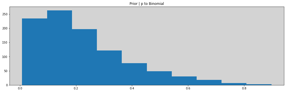
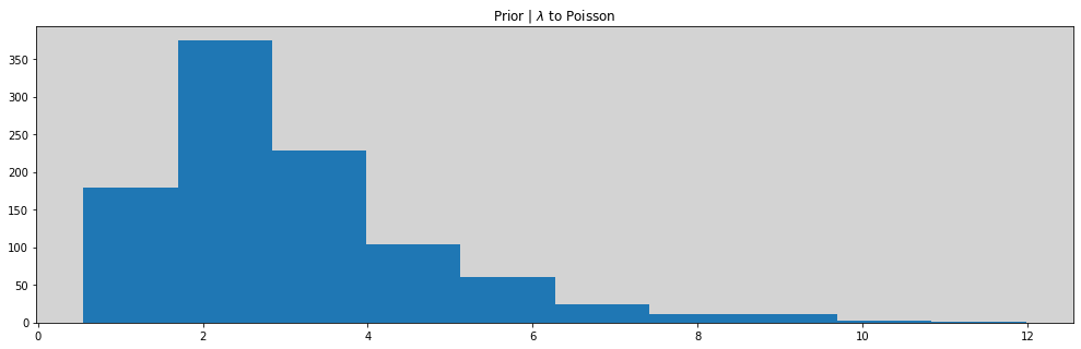
# Prioris
ap = np.random.normal(-1.5, 1, 1000)
al = np.random.normal(1, 0.5, 1000)

p = inv_logit(ap)
lam = np.exp(al)

plt.figure(figsize=(17, 5))
plt.hist(p)
plt.title('Prior | p to Binomial')
plt.show()

plt.figure(figsize=(17, 5))
plt.hist(lam)
plt.title('Prior | $\lambda$ to Poisson')
plt.show()
model = """
    data {
        int<lower=0> N;
        array[N] int<lower=0> y;
    }

    parameters {
        real al;
        real ap;
    }

    model {
        real p;
        real lambda;

        // Prior
        ap ~ normal(-1.5, 1);
        al ~ normal(1, 0.5);

        // Link functions
        p = inv_logit(ap);
        lambda = exp(al);

        // Likelihood
        for (i in 1:N){
            if (y[i] == 0) target += log_mix(p, 0, poisson_lpmf(0 | lambda));
            if (y[i] > 0)  target += log1m(p) + poisson_lpmf(y[i] | lambda);
        }
    }
"""

dat_list = {
    'N': len(y),
    'y': y,
}

posteriori = stan.build(model, data=dat_list)
samples = posteriori.sample(num_chains=4, num_samples=1000)
model_12_3 = az.from_pystan(
    posterior=samples,
    posterior_model=posteriori,
    observed_data=['y']
)
az.summary(model_12_3, hdi_prob=0.89)
| mean | sd | hdi_5.5% | hdi_94.5% | mcse_mean | mcse_sd | ess_bulk | ess_tail | r_hat | |
|---|---|---|---|---|---|---|---|---|---|
| al | -0.070 | 0.081 | -0.194 | 0.060 | 0.002 | 0.002 | 1431.0 | 1763.0 | 1.0 |
| ap | -1.983 | 0.526 | -2.791 | -1.208 | 0.014 | 0.010 | 1495.0 | 1810.0 | 1.0 |
R Code 12.10
print('Results: ')
print(' - p estimated: ', np.round(np.mean(inv_logit(model_12_3.posterior.ap.values.flatten())), 2), ' \t\t p original: ', prob_drink)
print(' - lambda estimated: ', np.round(np.mean(np.exp(model_12_3.posterior.al.values.flatten())), 2), ' \t estimated original: ', rate_work)
Results:
 - p estimated:  0.13  		 p original:  0.2
 - lambda estimated:  0.94  	 estimated original:  1
R Code 12.11
# This code is the same code that R Code 12.09
# In this book is stan version
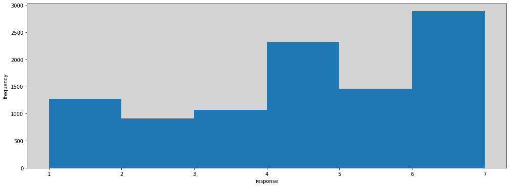
12.3 Ordered Categorical outcomes
12.3.2 Describing an ordered distribution with intercepts
R Code 12.12
df = pd.read_csv('./data/Trolley.csv', sep=';')
df
| case | response | order | id | age | male | edu | action | intention | contact | story | action2 | |
|---|---|---|---|---|---|---|---|---|---|---|---|---|
| 0 | cfaqu | 4 | 2 | 96;434 | 14 | 0 | Middle School | 0 | 0 | 1 | aqu | 1 |
| 1 | cfbur | 3 | 31 | 96;434 | 14 | 0 | Middle School | 0 | 0 | 1 | bur | 1 |
| 2 | cfrub | 4 | 16 | 96;434 | 14 | 0 | Middle School | 0 | 0 | 1 | rub | 1 |
| 3 | cibox | 3 | 32 | 96;434 | 14 | 0 | Middle School | 0 | 1 | 1 | box | 1 |
| 4 | cibur | 3 | 4 | 96;434 | 14 | 0 | Middle School | 0 | 1 | 1 | bur | 1 |
| ... | ... | ... | ... | ... | ... | ... | ... | ... | ... | ... | ... | ... |
| 9925 | ilpon | 3 | 23 | 98;299 | 66 | 1 | Graduate Degree | 0 | 1 | 0 | pon | 0 |
| 9926 | ilsha | 6 | 15 | 98;299 | 66 | 1 | Graduate Degree | 0 | 1 | 0 | sha | 0 |
| 9927 | ilshi | 7 | 7 | 98;299 | 66 | 1 | Graduate Degree | 0 | 1 | 0 | shi | 0 |
| 9928 | ilswi | 2 | 18 | 98;299 | 66 | 1 | Graduate Degree | 0 | 1 | 0 | swi | 0 |
| 9929 | nfrub | 2 | 17 | 98;299 | 66 | 1 | Graduate Degree | 1 | 0 | 0 | rub | 1 |
9930 rows × 12 columns
R Code 12.13
plt.figure(figsize=(17, 6))
plt.hist(df.response, bins=list(np.sort(df.response.unique())) )
plt.xlabel('response')
plt.ylabel('frequency')
plt.show()
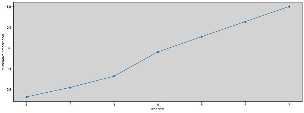
R Code 12.14
cum_pr_k = df.response.sort_values().value_counts(normalize=True, sort=False).cumsum()

plt.figure(figsize=(17, 6))
plt.plot(cum_pr_k, marker='o')
plt.xlabel('response')
plt.ylabel('cumulative proportional')

plt.show()
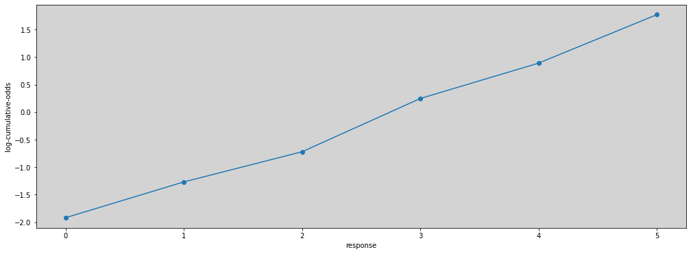
R Code 12.15
Where the \(\alpha_k\) is a “intercept” to all values of \(k\).
lco = [logit(cum_pr_k_i) for cum_pr_k_i in cum_pr_k ]
np.round(lco, 2)
/tmp/ipykernel_32026/1412855160.py:4: RuntimeWarning: invalid value encountered in log
  return np.log(p) - np.log(1 - p)
array([-1.92, -1.27, -0.72, 0.25, 0.89, 1.77, nan])
plt.figure(figsize=(17, 6))
plt.plot(lco[:-1], marker='o')
plt.xlabel('response')
plt.ylabel('log-cumulative-odds')
plt.show()
np.round([ inv_logit(l) for l in lco ], 2)
array([0.13, 0.22, 0.33, 0.56, 0.71, 0.85, nan])
RCode 12.16
1.8 Ordered logistic and probit regression (Stan Docs)
Ref: Stan - Docs
model = """
    data {
        int<lower=0> N;
        int<lower=2> K;
        array[N] int response;
    }

    parameters {
        ordered[K - 1] cutpoints;
    }

    model {
        cutpoints ~ normal(0, 1.5);

        for (i in 1:N){
            response[i] ~ ordered_logistic(0, cutpoints);
        }

    }
"""

dat_list = {
    'N': len(df),
    'K': len(df.response.unique()),
    'response': list(df.response.values),
}

posteriori = stan.build(model, data=dat_list)
samples = posteriori.sample(num_chains=4, num_samples=1000)
model_12_4 = az.from_pystan(
    posterior=samples,
    posterior_model=posteriori,
    observed_data=list(dat_list.keys()),
)
R Code 12.17
This code used quap intead of ulam and demonstre differences between.
R Code 12.18
az.summary(model_12_4, hdi_prob=0.89)
| mean | sd | hdi_5.5% | hdi_94.5% | mcse_mean | mcse_sd | ess_bulk | ess_tail | r_hat | |
|---|---|---|---|---|---|---|---|---|---|
| cutpoints[0] | -1.918 | 0.030 | -1.966 | -1.871 | 0.001 | 0.0 | 2717.0 | 2869.0 | 1.0 |
| cutpoints[1] | -1.267 | 0.024 | -1.305 | -1.228 | 0.000 | 0.0 | 3613.0 | 3488.0 | 1.0 |
| cutpoints[2] | -0.719 | 0.021 | -0.750 | -0.682 | 0.000 | 0.0 | 4018.0 | 3520.0 | 1.0 |
| cutpoints[3] | 0.247 | 0.020 | 0.216 | 0.279 | 0.000 | 0.0 | 4369.0 | 3136.0 | 1.0 |
| cutpoints[4] | 0.890 | 0.022 | 0.854 | 0.925 | 0.000 | 0.0 | 4106.0 | 3244.0 | 1.0 |
| cutpoints[5] | 1.770 | 0.029 | 1.724 | 1.816 | 0.000 | 0.0 | 4670.0 | 3467.0 | 1.0 |
R Code 12.19
az.plot_forest(model_12_4, combined=True, figsize=(17, 5), transform=inv_logit, hdi_prob=0.89)
plt.show()
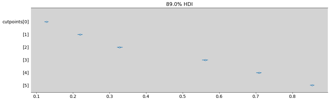
az.summary(inv_logit(model_12_4.posterior.cutpoints), hdi_prob=0.89)
| mean | sd | hdi_5.5% | hdi_94.5% | mcse_mean | mcse_sd | ess_bulk | ess_tail | r_hat | |
|---|---|---|---|---|---|---|---|---|---|
| cutpoints[0] | 0.128 | 0.003 | 0.123 | 0.133 | 0.0 | 0.0 | 2717.0 | 2869.0 | 1.0 |
| cutpoints[1] | 0.220 | 0.004 | 0.213 | 0.226 | 0.0 | 0.0 | 3613.0 | 3488.0 | 1.0 |
| cutpoints[2] | 0.328 | 0.005 | 0.321 | 0.336 | 0.0 | 0.0 | 4018.0 | 3520.0 | 1.0 |
| cutpoints[3] | 0.562 | 0.005 | 0.554 | 0.569 | 0.0 | 0.0 | 4369.0 | 3136.0 | 1.0 |
| cutpoints[4] | 0.709 | 0.005 | 0.701 | 0.716 | 0.0 | 0.0 | 4106.0 | 3244.0 | 1.0 |
| cutpoints[5] | 0.854 | 0.004 | 0.849 | 0.860 | 0.0 | 0.0 | 4670.0 | 3467.0 | 1.0 |