14 - Aventuras na Covariâncias¶

Imports, loadings and functions¶

import numpy as np

from scipy import stats

import matplotlib.pyplot as plt
from matplotlib.gridspec import GridSpec
from matplotlib.patches import Ellipse
import matplotlib.transforms as transforms

import pandas as pd

import networkx as nx
# from causalgraphicalmodels import CausalGraphicalModel

import arviz as az
# ArviZ ships with style sheets!
# https://python.arviz.org/en/stable/examples/styles.html#example-styles
az.style.use("arviz-darkgrid")

import xarray as xr

import stan
import nest_asyncio

plt.style.use('default')
plt.rcParams['axes.facecolor'] = 'lightgray'

# To DAG's
import daft
from causalgraphicalmodels import CausalGraphicalModel  # Just work in < python3.9 

# Add fonts to matplotlib to run xkcd

from matplotlib import font_manager

font_dirs = ["fonts/"]  # The path to the custom font file.
font_files = font_manager.findSystemFonts(fontpaths=font_dirs)

for font_file in font_files:
    font_manager.fontManager.addfont(font_file)

# To make plots like drawing 
# plt.xkcd()

# To running the stan in jupyter notebook
nest_asyncio.apply()

# https://matplotlib.org/stable/gallery/statistics/confidence_ellipse.html
def get_correlated_dataset(n, dependency, mu, scale):
    latent = np.random.randn(n, 2)
    dependent = latent.dot(dependency)
    scaled = dependent * scale
    scaled_with_offset = scaled + mu
    # return x and y of the new, correlated dataset
    return scaled_with_offset[:, 0], scaled_with_offset[:, 1]

# https://matplotlib.org/stable/gallery/statistics/confidence_ellipse.html
def confidence_ellipse(x, y, ax, n_std=3.0, facecolor='none', **kwargs):
    """
    Create a plot of the covariance confidence ellipse of *x* and *y*.

    Parameters
    ----------
    x, y : array-like, shape (n, )
        Input data.

    ax : matplotlib.axes.Axes
        The axes object to draw the ellipse into.

    n_std : float
        The number of standard deviations to determine the ellipse's radiuses.

    **kwargs
        Forwarded to `~matplotlib.patches.Ellipse`

    Returns
    -------
    matplotlib.patches.Ellipse
    """
    if x.size != y.size:
        raise ValueError("x and y must be the same size")

    cov = np.cov(x, y)
    pearson = cov[0, 1]/np.sqrt(cov[0, 0] * cov[1, 1])
    # Using a special case to obtain the eigenvalues of this
    # two-dimensional dataset.
    ell_radius_x = np.sqrt(1 + pearson)
    ell_radius_y = np.sqrt(1 - pearson)
    ellipse = Ellipse((0, 0), width=ell_radius_x * 2, height=ell_radius_y * 2,
                      facecolor=facecolor, **kwargs)

    # Calculating the standard deviation of x from
    # the squareroot of the variance and multiplying
    # with the given number of standard deviations.
    scale_x = np.sqrt(cov[0, 0]) * n_std
    #scale_x = n_std
    mean_x = np.mean(x)

    # calculating the standard deviation of y ...
    scale_y = np.sqrt(cov[1, 1]) * n_std
    #scale_y = n_std
    mean_y = np.mean(y)

    transf = transforms.Affine2D() \
        .rotate_deg(45) \
        .scale(scale_x, scale_y) \
        .translate(mean_x, mean_y)

    ellipse.set_transform(transf + ax.transData)
    return ax.add_patch(ellipse)

def draw_ellipse(mu, sigma, level, plot_points=None):
    
    fig, ax_nstd = plt.subplots(figsize=(17, 8))

    dependency_nstd = sigma.tolist()

    scale = 5, 5

    x, y = get_correlated_dataset(500, dependency_nstd, mu, scale)
    
    if plot_points is not None:
        ax_nstd.scatter(plot_points[:, 0], plot_points[:, 1], s=25)

    for l in level:
        confidence_ellipse(x, y, ax_nstd, n_std=l, edgecolor='black', alpha=0.3)

    # ax_nstd.scatter(mu[0], mu[1], c='red', s=3)
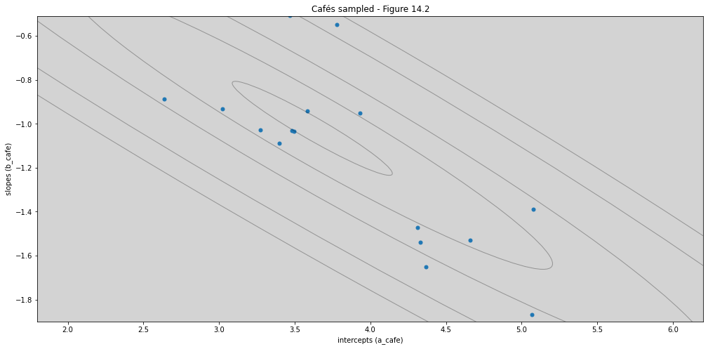
    ax_nstd.set_title('Cafés sampled - Figure 14.2')
    ax_nstd.set_xlabel('intercepts (a_cafe)')
    ax_nstd.set_ylabel('slopes (b_cafe)')
    
    ax_nstd.set_xlim(1.8, 6.2)
    ax_nstd.set_ylim(-1.9, -0.51)
    
    plt.show()

14.1 Varing Slopes by Contructions¶

R Code 14.1¶

a = 3.5        # Average morning wait time
b = (-1)       # Average difference afternoon wait time
sigma_a = 1    # std dev in intercepts
sigma_b = 0.5  # std in slopes
rho = (-0.7)   # correlation between intercepts and slopes

R Code 14.2¶

Mu = np.array([a, b])  # Vector
Mu

array([ 3.5, -1. ])

R Code 14.3¶

The matrix variance and covariance:

\[\begin{split} \begin{pmatrix} \mbox{variance of intercepts} & \mbox{covariance of intercepts & Slopes} \\ \mbox{covariance of intercepts & Slopes} & \mbox{variance of slopes} \end{pmatrix} \end{split}\]

And in math form:

\[\begin{split} \begin{pmatrix} \sigma^2_\alpha & \sigma_\alpha\sigma_\beta\rho \\ \sigma_\alpha\sigma_\beta\rho & \sigma^2_\beta \end{pmatrix} \end{split}\]

R Code 14.3¶

cov_ab = sigma_a * sigma_b * rho
Sigma = np.matrix([
    [sigma_a**2, cov_ab],
    [cov_ab, sigma_b**2]
])
Sigma

matrix([[ 1.  , -0.35],
        [-0.35,  0.25]])

R Code 14.4¶

np.matrix([[1,2], [3, 4]])

matrix([[1, 2],
        [3, 4]])

R Code 14.5¶

sigmas = np.array([sigma_a, sigma_b])  # Standart Deviations

sigmas

array([1. , 0.5])

Rho = np.matrix([
    [1, rho],
    [rho, 1]
])  # Correlation Matrix

Rho

matrix([[ 1. , -0.7],
        [-0.7,  1. ]])

# Multiply to get covariance matrix
Sigma = np.diag(sigmas) * Rho * np.diag(sigmas)

Sigma

matrix([[ 1.  , -0.35],
        [-0.35,  0.25]])

R Code 14.6¶

N_cafe = 20

R Code 14.7¶

np.random.seed(5)   # used to replicate example

vary_effects = stats.multivariate_normal(mean=Mu, cov=Sigma).rvs(N_cafe)
vary_effects

array([[ 3.02149593, -0.9304358 ],
       [ 1.05666673, -0.12762876],
       [ 3.58546284, -0.46432203],
       [ 4.3297356 , -1.53991745],
       [ 3.27332508, -1.02933771],
       [ 4.65859716, -1.5303893 ],
       [ 3.93018946, -0.9524405 ],
       [ 5.06625508, -1.869279  ],
       [ 2.58529637,  0.0287956 ],
       [ 5.07890482, -1.39033508],
       [ 4.36801698, -1.65042937],
       [ 4.31342478, -1.47263713],
       [ 2.59854231, -0.38835499],
       [ 3.39670791, -1.09000246],
       [ 3.48373345, -1.03170127],
       [ 2.63542057, -0.88644913],
       [ 3.49374238, -1.03389681],
       [ 3.58250316, -0.94285315],
       [ 3.46768242, -0.50699357],
       [ 3.77789108, -0.54770738]])

R Code 14.8¶

a_cafe = vary_effects[:, 0]  # Intercepts samples
b_cafe = vary_effects[:, 1]  # Slopes samples

R Code 14.9¶

levels = [0.1, 0.3, 0.5, 0.8, 0.99]
draw_ellipse(mu=Mu, sigma=Sigma, level=levels, plot_points=vary_effects)

Overthinking: We define the covariance with 3 parameters: (pag 440)

Firt variable standart deviations $\sigma_\alpha$
Second variable standart deviations $ \sigma_\beta $
Correlation between two variables $\rho_{\alpha\beta}$

Whu the covariance is equal to $\sigma_\alpha \sigma_\beta \rho_{\alpha\beta}$?

The usual definition of the covariance between two variables $x$ and $y$ is:

\[ cov(x, y) = \mathbb{E}(xy) - \mathbb{E}(x)\mathbb{E}(y) \]

To simple variance this concept is the same:

\[ var(x) = cov(x, x) = \mathbb{E}(x^2) - \mathbb{E}(x)^2\]

If the variable with only mean equal zero ($0$), then the variance to be:

\[ var(x) = cov(x) = \mathbb{E}(x^2), \mbox{ if the } \mathbb{E}(x) = 0 \]

The correlation live in $[-1, 1]$, this is only the covariance rescaled. To be rescaled covariance just:

\[ cov(xy) = \sqrt{var(x)var(y)} \rho_{xy} \]

or better:

\[ cov(xy) = \sigma_x \sigma_y \rho_{xy} \]

R Code 14.10¶

N_visit = 10

afternoon = np.tile([0, 1], reps=int((N_visit*N_cafe)/2))
cafe_id = np.repeat(np.arange(0, N_cafe), N_visit)

mu = a_cafe[cafe_id] + b_cafe[cafe_id]*afternoon
sigma = 0.5  # std dev within cafes

wait = np.random.normal(mu, sigma, size=N_visit*N_cafe)
cafe_id += 1  # index from 1 to 20 cafe_id, need to Stan index

d = pd.DataFrame({'cafe': cafe_id, 'afternoon':afternoon, 'wait': wait})
d

	cafe	afternoon	wait
0	1	0	2.713830
1	1	1	1.965617
2	1	0	3.261427
3	1	1	2.836598
4	1	0	3.105162
...	...	...	...
195	20	1	4.001264
196	20	0	3.991292
197	20	1	2.764103
198	20	0	3.507337
199	20	1	2.439118

200 rows × 3 columns

14.1.3 The varing slope model¶

The likelihood:

\[ W_i \sim Normal(\mu_i, \sigma) \]

and the linear model:

\[ \mu_i = \alpha_{CAFÉ[i]} + \beta_{CAFÉ[i]}A_i \]

Then comes the matrix of varing intercepts and slopes, with it’s covariance matrix:

Population of varying effects: $$

(1)¶\[\begin{bmatrix} \alpha_{CAFÉ} \\ \beta_{CAFÉ} \end{bmatrix}\]

\sim Normal

(2)¶\[\begin{pmatrix} \begin{bmatrix} \alpha \\ \beta \end{bmatrix}, S \end{pmatrix}\]

\[ \begin{align}\begin{aligned}construct covariance matrix:\\\begin{split}$$S = \begin{pmatrix} \sigma_\alpha & 0 \\ 0 & \sigma_\beta \end{pmatrix} R \begin{pmatrix} \sigma_\alpha & 0 \\ 0 & \sigma_\beta \end{pmatrix} \end{split}\end{aligned}\end{align} \]

The $R$ is the correlation matrix. In this simple case $R$ is defined like:

\[\begin{split} R = \begin{pmatrix} 1 & \rho \\ \rho & 1 \end{pmatrix} \end{split}\]

And the priors and hyper-priors:

prior for intercept:

\[ \alpha \sim Normal(5, 2) \]

prior for average slope:

\[ \beta \sim Normal(-1, 0.5) \]

prior for stddev within cafés

\[\sigma \sim Exponential(1) \]

prior for stddev among cafés

\[ \sigma_\alpha \sim Exponential(1) \]

prior for stddev among slopes

\[ \sigma_\beta \sim Exponential(1) \]

prior for correlation matrix

\[ R \sim LKJcorr(2) \]

R Code 14.11¶

# Dont have the function LKJcorr implemented in numpy or scipy
# Stan implementation - https://mc-stan.org/docs/functions-reference/lkj-correlation.html

R Code 14.12¶

# https://mc-stan.org/docs/stan-users-guide/multivariate-hierarchical-priors.html

model = """
    data {
        int N;
        int N_cafe;
        int N_periods;
        
        array[N] real wait;
        array[N] int cafe;
        array[N] int afternoon; 
    }
    
    parameters {
        real<lower=0> sigma;
        vector<lower=0>[2] sigma_cafe;
        
        vector[N_cafe] alpha_cafe;
        vector[N_cafe] beta_cafe;
        
        real alpha;  // Like bar_alpha (hyper-prior)
        real beta;   // Like bar_beta (hyper-prior)
        
        corr_matrix[N_periods] Rho;
    }
    
    model {
        vector[N] mu;
        vector[2] Y_cafe[N_cafe];
        vector[2] MU_cafe;
        
        //(sigma) - Prior to likelihood
        sigma ~ exponential(1);  
        
        
        // (sigma_cafe) - Hyper Prior
        sigma_cafe ~ exponential(1);
        
        // (Rho) - Hyper Prior
        Rho ~ lkj_corr(2);
        
        // (MU_cafe) - Hyper Prior
        alpha ~ normal(5, 2);
        beta ~ normal(-1, 0.5);
  
        MU_cafe = [alpha, beta]';
        
        // (alpha_cafe, beta_cafe) - Prior 
        for (j in 1:N_cafe){
            Y_cafe[j] = [alpha_cafe[j], beta_cafe[j]]' ; 
        }
        
        Y_cafe ~ multi_normal(MU_cafe, quad_form_diag(Rho, sigma_cafe));  // Prior to alpha_cafe and beta_cafe
    
    
        // (mu) - Linear model
        for (i in 1:N){
            mu[i] = alpha_cafe[ cafe[i] ] + beta_cafe[ cafe[i] ] * afternoon[i];
        }
        
        // Likelihood 
        wait ~ normal(mu, sigma);
    }
"""

dat_list = {
    'N': len(d),
    'N_cafe': N_cafe,
    'N_periods': len(d.afternoon.unique()),
    'wait':  d.wait.values,
    'afternoon': d.afternoon.values,
    'cafe': d.cafe.values,
}

posteriori = stan.build(model, data=dat_list)
samples = posteriori.sample(num_chains=4, num_samples=1000)

model_another_way = """
    data {
        int N;
        int N_cafe;
        int N_periods;
        
        array[N] real wait;
        array[N] int cafe;
        array[N] int afternoon; 
    }
    
    parameters {
        real<lower=0> sigma;
        vector<lower=0>[2] sigma_cafe;
        
        vector[N_cafe] alpha_cafe;
        vector[N_cafe] beta_cafe;
        
        real alpha;  // Like bar_alpha (hyper-prior)
        real beta;   // Like bar_beta (hyper-prior)
        
        corr_matrix[N_periods] Rho;
    }
    
    model {
        vector[N] mu;
        
        //(sigma) - Prior to likelihood
        sigma ~ exponential(1);  
        
        
        // (sigma_cafe) - Hyper Prior
        sigma_cafe ~ exponential(1);
        
        // (Rho) - Hyper Prior
        Rho ~ lkj_corr(2);
        
        // (MU_cafe) - Hyper Prior
        alpha ~ normal(5, 2);
        beta ~ normal(-1, 0.5);

        for (i in 1:N_cafe){
            [alpha_cafe[i], beta_cafe[i]]' ~ multi_normal([alpha, beta]', quad_form_diag(Rho, sigma_cafe));
        }
        
    
        // (mu) - Linear model
        for (i in 1:N){
            mu[i] = alpha_cafe[ cafe[i] ] + beta_cafe[ cafe[i] ] * afternoon[i];
        }
        
        // Likelihood 
        wait ~ normal(mu, sigma);
    }
"""

m14_1 = az.from_pystan(
    posterior=samples,
    posterior_model=posteriori,
    observed_data=dat_list.keys()
)

az.summary(m14_1, hdi_prob=0.89)

/home/rodolpho/Projects/bayesian/BAYES/lib/python3.8/site-packages/arviz/stats/diagnostics.py:592: RuntimeWarning: invalid value encountered in double_scalars
  (between_chain_variance / within_chain_variance + num_samples - 1) / (num_samples)

	mean	sd	hdi_5.5%	hdi_94.5%	mcse_mean	mcse_sd	ess_bulk	ess_tail	r_hat
sigma	0.494	0.027	0.454	0.541	0.000	0.000	5147.0	3085.0	1.0
sigma_cafe[0]	0.955	0.163	0.695	1.187	0.002	0.002	5092.0	3241.0	1.0
sigma_cafe[1]	0.454	0.107	0.281	0.616	0.002	0.002	2209.0	1995.0	1.0
alpha_cafe[0]	2.944	0.204	2.608	3.259	0.003	0.002	5598.0	3371.0	1.0
alpha_cafe[1]	1.102	0.213	0.766	1.445	0.003	0.002	5163.0	3691.0	1.0
alpha_cafe[2]	3.714	0.208	3.384	4.043	0.003	0.002	4668.0	2735.0	1.0
alpha_cafe[3]	4.153	0.199	3.807	4.447	0.003	0.002	5745.0	3062.0	1.0
alpha_cafe[4]	3.306	0.203	2.976	3.615	0.003	0.002	4642.0	3251.0	1.0
alpha_cafe[5]	4.836	0.202	4.486	5.135	0.003	0.002	5839.0	3544.0	1.0
alpha_cafe[6]	4.259	0.203	3.948	4.598	0.003	0.002	5354.0	3489.0	1.0
alpha_cafe[7]	4.835	0.215	4.478	5.165	0.003	0.002	4494.0	3171.0	1.0
alpha_cafe[8]	2.744	0.206	2.436	3.075	0.003	0.002	5784.0	2714.0	1.0
alpha_cafe[9]	5.194	0.204	4.869	5.515	0.003	0.002	4640.0	3116.0	1.0
alpha_cafe[10]	3.951	0.205	3.654	4.303	0.003	0.002	4219.0	2878.0	1.0
alpha_cafe[11]	4.524	0.208	4.181	4.844	0.003	0.002	5084.0	3117.0	1.0
alpha_cafe[12]	2.557	0.202	2.230	2.881	0.003	0.002	4584.0	2660.0	1.0
alpha_cafe[13]	3.554	0.210	3.198	3.864	0.003	0.002	4083.0	2590.0	1.0
alpha_cafe[14]	3.806	0.202	3.487	4.124	0.003	0.002	5093.0	3223.0	1.0
alpha_cafe[15]	2.686	0.206	2.354	3.012	0.003	0.002	4761.0	3236.0	1.0
alpha_cafe[16]	3.537	0.202	3.228	3.880	0.003	0.002	5647.0	3117.0	1.0
alpha_cafe[17]	3.514	0.204	3.171	3.821	0.003	0.002	5429.0	3417.0	1.0
alpha_cafe[18]	3.718	0.205	3.395	4.041	0.003	0.002	5135.0	3168.0	1.0
alpha_cafe[19]	3.453	0.202	3.135	3.776	0.003	0.002	5510.0	3590.0	1.0
beta_cafe[0]	-0.766	0.234	-1.154	-0.414	0.003	0.002	5345.0	3726.0	1.0
beta_cafe[1]	-0.119	0.275	-0.549	0.324	0.004	0.004	4223.0	2961.0	1.0
beta_cafe[2]	-0.686	0.259	-1.080	-0.271	0.004	0.003	3532.0	2484.0	1.0
beta_cafe[3]	-1.178	0.231	-1.534	-0.799	0.003	0.002	5704.0	2683.0	1.0
beta_cafe[4]	-0.863	0.228	-1.222	-0.490	0.003	0.002	4366.0	3321.0	1.0
beta_cafe[5]	-1.450	0.238	-1.821	-1.070	0.003	0.002	5271.0	3484.0	1.0
beta_cafe[6]	-1.378	0.240	-1.762	-0.991	0.004	0.003	4525.0	3184.0	1.0
beta_cafe[7]	-1.673	0.263	-2.112	-1.267	0.004	0.003	3798.0	3061.0	1.0
beta_cafe[8]	-0.619	0.243	-1.024	-0.248	0.003	0.003	5271.0	3084.0	1.0
beta_cafe[9]	-1.446	0.253	-1.856	-1.047	0.004	0.003	4326.0	2741.0	1.0
beta_cafe[10]	-1.324	0.245	-1.719	-0.944	0.004	0.003	3760.0	2877.0	1.0
beta_cafe[11]	-1.421	0.243	-1.819	-1.054	0.004	0.003	4647.0	3288.0	1.0
beta_cafe[12]	-0.591	0.239	-0.978	-0.216	0.003	0.002	4727.0	3014.0	1.0
beta_cafe[13]	-1.357	0.265	-1.749	-0.909	0.005	0.004	2824.0	2721.0	1.0
beta_cafe[14]	-1.045	0.229	-1.428	-0.709	0.003	0.002	5144.0	3521.0	1.0
beta_cafe[15]	-0.826	0.244	-1.234	-0.458	0.004	0.003	4317.0	3206.0	1.0
beta_cafe[16]	-0.966	0.234	-1.344	-0.607	0.003	0.002	4929.0	3126.0	1.0
beta_cafe[17]	-0.826	0.241	-1.220	-0.445	0.003	0.002	5018.0	3167.0	1.0
beta_cafe[18]	-0.821	0.244	-1.203	-0.425	0.004	0.003	4382.0	2956.0	1.0
beta_cafe[19]	-0.640	0.251	-1.071	-0.268	0.004	0.003	3712.0	3520.0	1.0
alpha	3.632	0.216	3.293	3.972	0.003	0.002	4168.0	3264.0	1.0
beta	-1.003	0.120	-1.196	-0.814	0.002	0.001	3412.0	3079.0	1.0
Rho[0, 0]	1.000	0.000	1.000	1.000	0.000	0.000	4000.0	4000.0	NaN
Rho[0, 1]	-0.743	0.142	-0.961	-0.553	0.003	0.002	2243.0	1976.0	1.0
Rho[1, 0]	-0.743	0.142	-0.961	-0.553	0.003	0.002	2243.0	1976.0	1.0
Rho[1, 1]	1.000	0.000	1.000	1.000	0.000	0.000	3969.0	3852.0	1.0

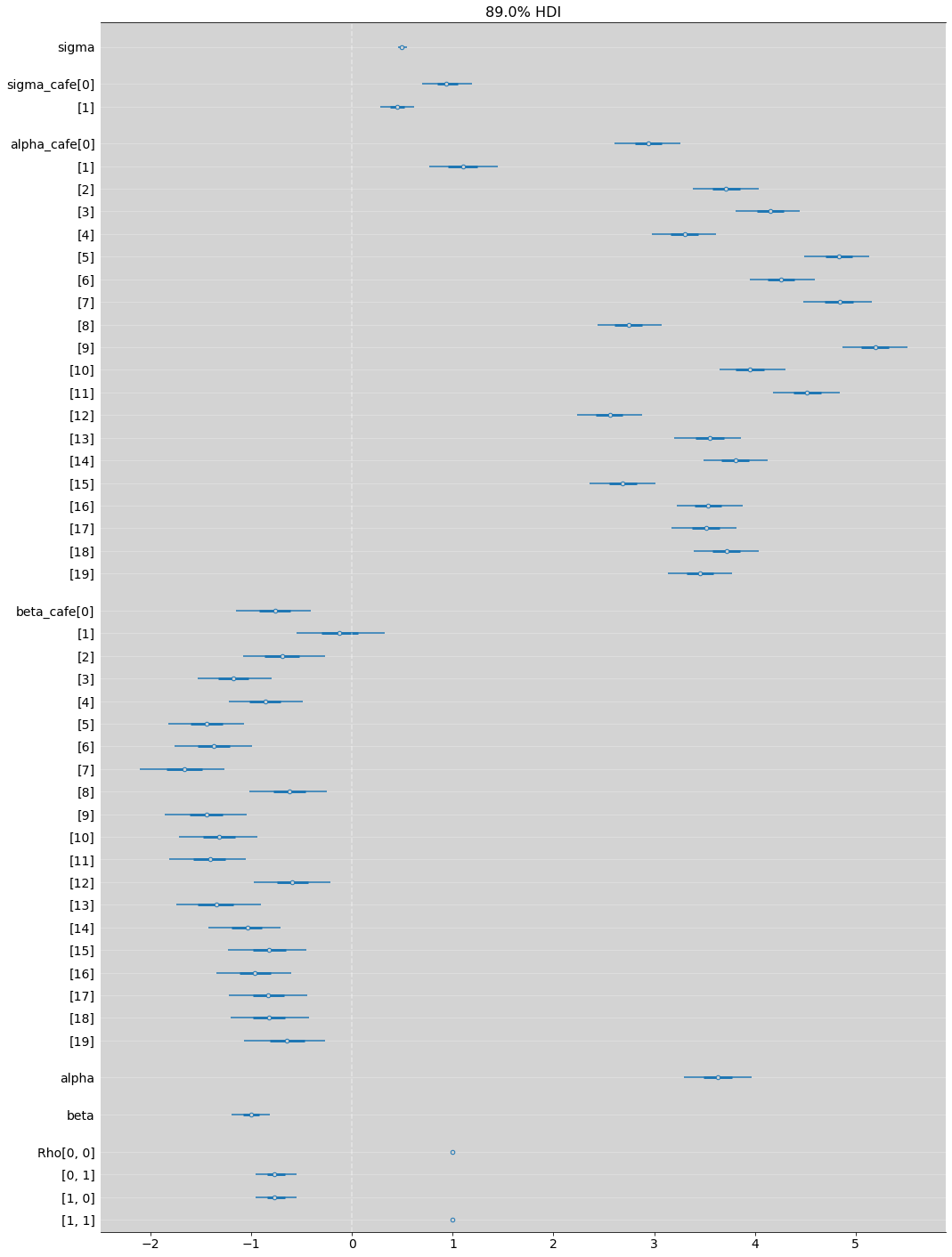
az.plot_forest(m14_1, hdi_prob=0.89, combined=True, figsize=(17, 25))
plt.grid(axis='y', color='white', alpha=0.3)
plt.axvline(x=0, ls='--', color='white', alpha=0.4)
plt.show()

R Code 14.13¶

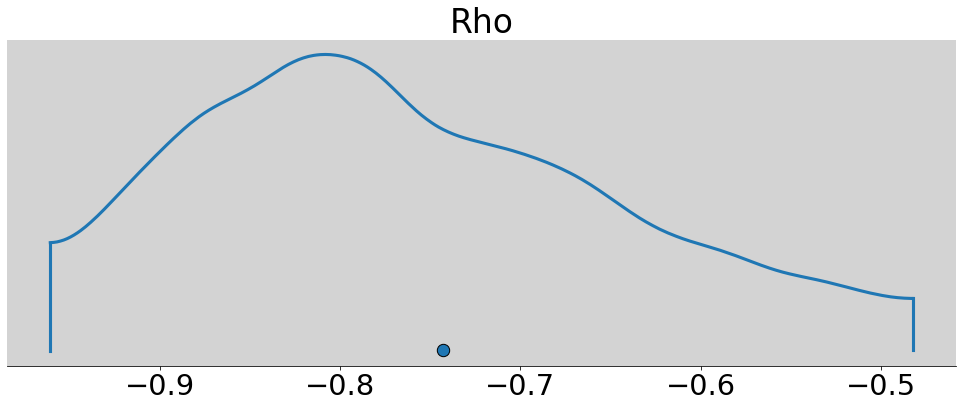
az.plot_density(m14_1.posterior.Rho.sel(Rho_dim_0=0, Rho_dim_1=1), figsize=(17, 6))
plt.xlabel = 'Correlation'
plt.ylabel = 'Density'
plt.show()

R Code 14.14 & R Code 14.15¶

post_alpha = m14_1.posterior.alpha.mean().values
post_beta = m14_1.posterior.beta.mean().values

post_sigma_alpha = m14_1.posterior.sigma_cafe.sel(sigma_cafe_dim_0=0).mean().values
post_sigma_beta = m14_1.posterior.sigma_cafe.sel(sigma_cafe_dim_0=1).mean().values
post_rho = m14_1.posterior.Rho.sel(Rho_dim_0=0, Rho_dim_1=1).mean().values

print('Posterior alpha:', post_alpha)
print('Posterior beta:', post_beta)
print('Posterior sigma alpha:', post_sigma_alpha)
print('Posterior sigma beta:', post_sigma_beta)
print('Posterior Rho:', post_rho)

Posterior alpha: 3.6320048659560236
Posterior beta: -1.0031288413854578
Posterior sigma alpha: 0.9549508114681846
Posterior sigma beta: 0.4542529928057041
Posterior Rho: -0.7428039489326627

post_matrix_sigma_alpha_beta = np.matrix([[post_sigma_alpha, 0],[0, post_sigma_beta]])
post_matrix_sigma_alpha_beta

matrix([[0.95495081, 0.        ],
        [0.        , 0.45425299]])

post_matrix_rho = np.matrix([[1, post_rho],[post_rho, 1]])
post_matrix_rho

matrix([[ 1.        , -0.74280395],
        [-0.74280395,  1.        ]])

post_Sigma = post_matrix_sigma_alpha_beta * post_matrix_rho * post_matrix_sigma_alpha_beta
post_Sigma

matrix([[ 0.91193105, -0.32222038],
        [-0.32222038,  0.20634578]])

a1 = [d.loc[(d['afternoon'] == 0) & (d['cafe'] == i)]['wait'].mean() for i in range(1, N_cafe+1)]
b1 = [d.loc[(d['afternoon'] == 1) & (d['cafe'] == i)]['wait'].mean() for i in range(1, N_cafe+1)]

# Remember that in R Code 14.1 above, the data is build as
# a = 3.5        # Average morning wait time
# b = (-1)       # Average difference afternoon wait time
# because this, b value is b - a, like this

b1 = [b1[i] - a1[i] for i in range(len(a1))]

# Extract posterior means of partially polled estimates
a2 = [m14_1.posterior.alpha_cafe.sel(alpha_cafe_dim_0=i).mean().values for i in range(N_cafe)]
b2 = [m14_1.posterior.beta_cafe.sel(beta_cafe_dim_0=i).mean().values for i in range(N_cafe)]

fig, ax_nstd = plt.subplots(figsize=(17, 8))

mu = np.array([post_alpha, post_beta])
dependency_nstd = post_Sigma.tolist()

scale = 5, 5

level = [0.1, 0.3, 0.5, 0.8, 0.99]

x, y = get_correlated_dataset(500, dependency_nstd, mu, scale)

ax_nstd.scatter(a1, b1, s=25, color='b')
ax_nstd.scatter(a2, b2, s=25, facecolor='gray')

ax_nstd.plot([a1, a2], [b1, b2], 'k-', linewidth=0.5)
    
for l in level:
    confidence_ellipse(x, y, ax_nstd, n_std=l, edgecolor='black', alpha=0.3)

# ax_nstd.scatter(mu[0], mu[1], c='red', s=3)
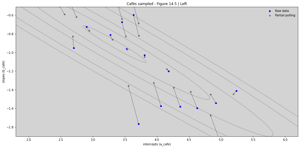
ax_nstd.set_title('Cafés sampled - Figure 14.5 | Left')
ax_nstd.set_xlabel('intercepts (a_cafe)')
ax_nstd.set_ylabel('slopes (b_cafe)')

ax_nstd.set_xlim(1.8, 6.2)
ax_nstd.set_ylim(-1.9, -0.51)

# ax_nstd.legend()
ax_nstd.legend(['Raw data', 'Partial polling'])

plt.plot(1,2, c='r')

plt.show()

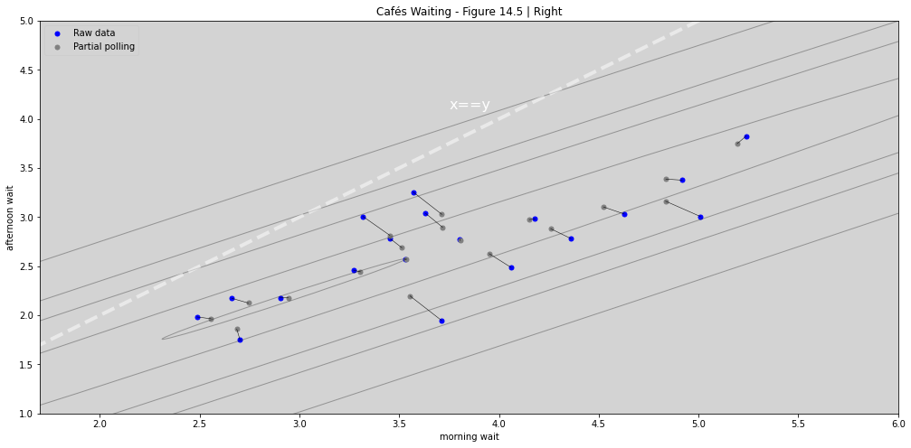
R Code 14.16 & R Code 14.17¶

wait_morning_1 = (a1)
wait_afternoon_1 = [sum(x) for x in zip(a1, b1)]
wait_morning_2 = (a2)
wait_afternoon_2 = [sum(x) for x in zip(a2, b2)]

# now shrinkage distribution by simulation  

v = np.random.multivariate_normal(mu ,post_Sigma, 1000)
v[:, 1] = [sum(x) for x in v]  # calculation afternoon wait
Sigma_est2 = np.cov(v[:, 0], v[:, 1])

mu_est2 = [0, 0]  # Empty vector mu
mu_est2[0] = mu[0] 
mu_est2[1] = mu[0] + mu[1]

fig, ax_nstd = plt.subplots(figsize=(17, 8))

scale = 5, 5
#level = [0.1, 0.3, 0.5, 0.8, 0.99]
level = [0.1, 0.69, 1.5, 2.0, 3.0]

dependency_nstd = Sigma_est2.tolist()
x, y = get_correlated_dataset(500, dependency_nstd, mu_est2, scale)

ax_nstd.scatter(wait_morning_1, wait_afternoon_1, s=25, color='b')
ax_nstd.scatter(wait_morning_2, wait_afternoon_2, s=25, facecolor='gray')

ax_nstd.plot([wait_morning_1, wait_morning_2],
             [wait_afternoon_1, wait_afternoon_2], 
             'k-', linewidth=0.5)

for l in level:
    confidence_ellipse(x, y, ax_nstd, n_std=l, edgecolor='black', alpha=0.3)

ax_nstd.set_title('Cafés Waiting - Figure 14.5 | Right')
ax_nstd.set_xlabel('morning wait')
ax_nstd.set_ylabel('afternoon wait')

ax_nstd.plot([0, 10], [0, 10], ls='--', color='white', alpha=0.5, linewidth=4)
ax_nstd.text(3.75, 4.1, "x==y",color='white', fontsize=16)

ax_nstd.set_xlim(1.7, 6)
ax_nstd.set_ylim(1, 5)

# ax_nstd.legend()
ax_nstd.legend(['Raw data', 'Partial polling'])

plt.plot(1,2, c='r')

plt.show()

14.2 Advanced varing Slopes¶

R Code 14.18¶

# Previous chimpanzees models is in chapter 11

df = pd.read_csv('./data/chimpanzees.csv', sep=';')

# Build the treatment data
df['treatment'] = 1 + df['prosoc_left'] + 2 * df['condition']  
df.head(20)

	actor	recipient	block	trial	prosoc_left	chose_prosoc	pulled_left	treatment
0	1	NaN	1	2	0	1	0	1
1	1	NaN	1	4	0	0	1	1
2	1	NaN	1	6	1	0	0	2
3	1	NaN	1	8	0	1	0	1
4	1	NaN	1	10	1	1	1	2
5	1	NaN	1	12	1	1	1	2
6	1	NaN	2	14	1	0	0	2
7	1	NaN	2	16	1	0	0	2
8	1	NaN	2	18	0	1	0	1
9	1	NaN	2	20	0	1	0	1
10	1	NaN	2	22	0	0	1	1
11	1	NaN	2	24	1	0	0	2
12	1	NaN	3	26	0	0	1	1
13	1	NaN	3	28	1	1	1	2
14	1	NaN	3	30	0	1	0	1
15	1	NaN	3	32	1	1	1	2
16	1	NaN	3	34	1	0	0	2
17	1	NaN	3	36	0	1	0	1
18	1	NaN	4	38	1	1	1	2
19	1	NaN	4	40	0	0	1	1

df.tail(20)

	actor	recipient	condition	block	trial	prosoc_left	chose_prosoc	pulled_left	treatment
484	7	2.0	1	3	34	0	0	1	3
485	7	3.0	1	3	36	1	1	1	4
486	7	7.0	1	4	38	0	0	1	3
487	7	2.0	1	4	40	0	0	1	3
488	7	4.0	1	4	42	1	1	1	4
489	7	5.0	1	4	44	0	0	1	3
490	7	6.0	1	4	46	0	0	1	3
491	7	3.0	1	4	48	0	0	1	3
492	7	5.0	1	5	50	1	1	1	4
493	7	4.0	1	5	52	0	0	1	3
494	7	3.0	1	5	54	0	0	1	3
495	7	2.0	1	5	56	1	1	1	4
496	7	6.0	1	5	58	1	1	1	4
497	7	7.0	1	5	60	1	1	1	4
498	7	5.0	1	6	62	1	1	1	4
499	7	4.0	1	6	64	1	1	1	4
500	7	6.0	1	6	66	1	1	1	4
501	7	3.0	1	6	68	0	0	1	3
502	7	7.0	1	6	70	0	0	1	3
503	7	2.0	1	6	72	0	0	1	3

\[ L_i \sim Binomial(1, p_i) \]

\[ logit(p_i) = \gamma_{_{TID}[i]} + \alpha_{_{ACTOR}[I], _{TID}[I]} + \beta_{_{BLOCK}[I], _{TID}[I]} \]

\[\gamma_{_{TID}} \sim Normal(0, 1)\]

\[\begin{split}\begin{bmatrix} \alpha_{j, 1} \\ \alpha_{j, 2} \\ \alpha_{j, 3} \\ \alpha_{j, 4} \end{bmatrix} \sim MVNormal \begin{pmatrix} \begin{bmatrix} 0 \\ 0 \\ 0 \\ 0 \end{bmatrix} , S_{_{ACTOR}} \end{pmatrix}\end{split}\]

\[\begin{split}\begin{bmatrix} \beta_{j, 1} \\ \beta_{j, 2} \\ \beta_{j, 3} \\ \beta_{j, 4} \end{bmatrix} \sim MVNormal \begin{pmatrix} \begin{bmatrix} 0 \\ 0 \\ 0 \\ 0 \end{bmatrix} , S_{_{BLOCK}} \end{pmatrix}\end{split}\]

Hyper-prior to $S_{_{ACTOR}}$:

\[\sigma_{_{ACTOR}} \sim Exponential(1)\]

\[ \rho_{_{ACTOR}} \sim dlkjcorr(4) \]

Hyper-prior to $S_{_{BLOCK}}$: $$ \sigma_{_{BLOCK}} \sim Exponential(1) $$

\[ \rho_{_{BLOCK}} \sim dlkjcorr(4) \]

This is essentially an interaction model that allow the effect of each treatment to vary by actor and each block.

Important features to understanding this model¶

5.1 Overview of data types¶

Array types (stan docs link)¶

array[10] real x;
array[6, 7] matrix[3, 3] m;
array[12, 8, 15] complex z;

declares $x$ to be a one-dimensional array of size $10$ containing real values.
declares $m$ to be a two-dimensional array of size $[6 \times 7]$ containing values that are $[3 \times 3]$ matrices .
declares $z$ to be a $[12 \times 8 \times 15]$ array of complex numbers.

And read this two parts below

5.5 Vector and matrix data types ¶

Stan provides three types of container objects: arrays, vectors, and matrices.

5.6 Array data type ¶

Stan supports arrays of arbitrary dimension.

Depreciated Features in Stan to build this example:¶

13.10 Brackets array syntax

After Stan 2.26 the declarations below:

int n[5];
real a[3, 4];
real<lower=0> z[5, 4, 2];
vector[7] mu[3];
matrix[7, 2] mu[15, 12];
cholesky_factor_cov[5, 6] mu[2, 3, 4];

was replaced to:

array[5] int n;
array[3, 4] real a;
array[5, 4, 2] real<lower=0> z;
array[3] vector[7] mu;
array[15, 12] matrix[7, 2] mu;
array[2, 3, 4] cholesky_factor_cov[5, 6] mu;

13.12 Nested multiple indexing in assignments

This statements

a[:][1] = b;

was replaced by

a[:, 1] = b;

Explanation:¶

Why this alpha ~ multi_normal(rep_vector(0, 4), quad_form_diag(Rho_actor, sigma_actor)); works in code below?

Response:¶

Let be the code:

parameters{
    ...
   vector[qty_treatments] gamma;
   ...
}

There are $4$ positions in vector gamma, then when we atrribute the normal(0, 1), we realize make the broadcast:

gamma ~ normal(0, 1);

is equivalent to:

for (i in 1:qty_treatments){
    gamma[i] ~ normal(0, 1);
}

This is the same reason that code with multi_normal works. Let see this in more details:

parameters{
    ...
   array[qty_chimpanzees] vector[qty_treatments] alpha;
   ...
}

Now, the alpha have two dimensional structure.

Note: index in Stan start in 1, not in zero like python.

The alpha[1, 1] is alpha to chimpanzees=1 and to treatment=1
The alpha[1, 2] is alpha to chimpanzees=1 and to treatment=2
The alpha[2, 3] is alpha to chimpanzees=2 and to treatment=3
The alpha[7, 4] is alpha to chimpanzees=7 and to treatment=4

And

The alpha[1, :] is alpha to chimpanzees=1 and to all treatments

The type of data to alpha[1, :] is a vector[qty_treatments].

This is the same type that multi_normal expected to attribuite the results.

Then, the code works!

model = """
    data {
        int N;
        int qty_chimpanzees;
        int qty_blocks;
        int qty_treatments;
        
        array[N] int pulled_left;
        array[N] int actor;
        array[N] int block;
        array[N] int treatment;
    }
    
    parameters{
        vector[qty_treatments] gamma;
        array[qty_chimpanzees] vector[qty_treatments] alpha;
        array[qty_blocks] vector[qty_treatments] beta;
        
        corr_matrix[qty_treatments] Rho_actor;
        vector<lower=0>[qty_treatments] sigma_actor;
        
        corr_matrix[qty_treatments] Rho_block;
        vector[qty_treatments] sigma_block;
    }
    
    model {
        vector[N] p;
        
        // Fixed Priors
        Rho_actor ~ lkj_corr(4);
        sigma_actor ~ exponential(1);
        
        Rho_block ~ lkj_corr(4);
        sigma_block ~ exponential(1);
        
    
        // Adaptatives Priors
        gamma ~ normal(0, 1);
        
        alpha ~ multi_normal(rep_vector(0, 4), quad_form_diag(Rho_actor, sigma_actor));
        beta ~ multi_normal(rep_vector(0, 4), quad_form_diag(Rho_block, sigma_block));
        
        
        // Linear model
        for (i in 1:N){
            p[i] = gamma[ treatment[i] ] + alpha[ actor[i], treatment[i] ] + beta[ block[i], treatment[i] ];
            p[i] = inv_logit(p[i]);  // Link function
        }
    
    
        // Likelihood
        pulled_left ~ binomial(1, p);
    }
 
"""


dat_list = df[['pulled_left', 'actor', 'block', 'treatment']].to_dict('list')
dat_list['N'] = len(df)
dat_list['qty_chimpanzees'] = len(df['actor'].unique())
dat_list['qty_blocks'] = len(df['block'].unique())
dat_list['qty_treatments'] = len(df['treatment'].unique())

posteriori = stan.build(model, data=dat_list)
samples = posteriori.sample(num_chains=4, num_samples=1000)

m_14_2 = az.from_pystan(
    posterior=samples,
    posterior_model=posteriori,
    observed_data=dat_list.keys()
)

print(az.summary(m_14_2).to_string())

/home/rodolpho/Projects/bayesian/BAYES/lib/python3.8/site-packages/arviz/stats/diagnostics.py:592: RuntimeWarning: invalid value encountered in double_scalars
  (between_chain_variance / within_chain_variance + num_samples - 1) / (num_samples)
/home/rodolpho/Projects/bayesian/BAYES/lib/python3.8/site-packages/arviz/stats/diagnostics.py:592: RuntimeWarning: invalid value encountered in double_scalars
  (between_chain_variance / within_chain_variance + num_samples - 1) / (num_samples)

                  mean     sd  hdi_3%  hdi_97%  mcse_mean  mcse_sd  ess_bulk  ess_tail  r_hat
gamma[0]         0.191  0.528  -0.741    1.254      0.034    0.024     229.0     444.0   1.04
gamma[1]         0.669  0.409  -0.141    1.366      0.021    0.015     353.0     800.0   1.02
gamma[2]         0.027  0.588  -1.045    1.192      0.039    0.028     231.0     242.0   1.01
gamma[3]         0.618  0.580  -0.546    1.639      0.034    0.026     288.0     282.0   1.01
alpha[0, 0]     -0.860  0.660  -2.257    0.235      0.040    0.030     275.0     302.0   1.03
alpha[0, 1]     -0.540  0.481  -1.472    0.334      0.020    0.015     574.0     758.0   1.01
alpha[0, 2]     -0.964  0.716  -2.409    0.406      0.040    0.030     329.0     362.0   1.01
alpha[0, 3]     -0.537  0.683  -1.698    0.813      0.040    0.034     308.0     435.0   1.01
alpha[1, 0]      3.124  1.366   1.057    5.688      0.080    0.062     346.0     170.0   1.02
alpha[1, 1]      2.046  1.087   0.447    4.116      0.046    0.034     545.0     524.0   1.01
alpha[1, 2]      4.042  1.512   1.278    6.895      0.077    0.055     370.0     346.0   1.01
alpha[1, 3]      3.206  1.562   0.730    5.942      0.081    0.058     335.0     197.0   1.00
alpha[2, 0]     -1.119  0.659  -2.436   -0.053      0.038    0.027     305.0     576.0   1.01
alpha[2, 1]     -0.290  0.531  -1.222    0.710      0.029    0.021     310.0     280.0   1.01
alpha[2, 2]     -1.562  0.764  -2.987   -0.035      0.039    0.027     386.0     651.0   1.01
alpha[2, 3]     -1.201  0.684  -2.455    0.016      0.036    0.025     363.0     906.0   1.01
alpha[3, 0]     -0.917  0.641  -2.132    0.234      0.028    0.020     533.0     599.0   1.02
alpha[3, 1]     -0.585  0.477  -1.479    0.239      0.023    0.017     423.0     655.0   1.01
alpha[3, 2]     -1.927  0.809  -3.411   -0.390      0.046    0.032     304.0     366.0   1.00
alpha[3, 3]     -0.904  0.691  -2.166    0.379      0.042    0.030     264.0     479.0   1.01
alpha[4, 0]     -0.863  0.656  -2.149    0.370      0.040    0.028     280.0     347.0   1.02
alpha[4, 1]     -0.403  0.471  -1.318    0.465      0.018    0.014     661.0     918.0   1.01
alpha[4, 2]     -0.991  0.760  -2.466    0.387      0.048    0.034     255.0     402.0   1.01
alpha[4, 3]     -0.646  0.684  -1.940    0.572      0.040    0.028     298.0     595.0   1.01
alpha[5, 0]      0.882  0.644  -0.373    2.055      0.031    0.022     407.0     675.0   1.02
alpha[5, 1]     -0.097  0.494  -0.961    0.854      0.025    0.018     383.0     784.0   1.01
alpha[5, 2]      0.190  0.730  -1.287    1.439      0.049    0.035     229.0     198.0   1.02
alpha[5, 3]     -0.107  0.698  -1.398    1.155      0.045    0.032     242.0     154.0   1.02
alpha[6, 0]      1.095  0.690  -0.242    2.356      0.040    0.029     287.0     431.0   1.01
alpha[6, 1]      0.914  0.617  -0.204    2.085      0.057    0.045     141.0      87.0   1.04
alpha[6, 2]      2.632  0.937   1.073    4.521      0.046    0.032     424.0     654.0   1.01
alpha[6, 3]      2.684  1.296   0.514    5.052      0.078    0.058     288.0     343.0   1.01
beta[0, 0]      -0.099  0.334  -0.817    0.501      0.013    0.009     581.0     841.0   1.01
beta[0, 1]      -0.054  0.327  -0.811    0.536      0.012    0.009     750.0     906.0   1.00
beta[0, 2]      -0.065  0.287  -0.618    0.473      0.011    0.008     611.0     811.0   1.02
beta[0, 3]      -0.441  0.509  -1.501    0.289      0.029    0.021     346.0     300.0   1.01
beta[1, 0]       0.075  0.349  -0.595    0.763      0.018    0.013     413.0     365.0   1.02
beta[1, 1]      -0.148  0.358  -0.854    0.500      0.018    0.013     474.0     547.0   1.01
beta[1, 2]       0.085  0.302  -0.478    0.664      0.012    0.009     451.0     745.0   1.01
beta[1, 3]       0.182  0.375  -0.488    0.855      0.018    0.014     489.0     748.0   1.01
beta[2, 0]       0.356  0.467  -0.228    1.361      0.032    0.023     275.0     281.0   1.01
beta[2, 1]      -0.241  0.385  -1.043    0.359      0.024    0.017     317.0     457.0   1.01
beta[2, 2]       0.011  0.312  -0.559    0.599      0.012    0.009     539.0     584.0   1.01
beta[2, 3]       0.166  0.401  -0.502    1.010      0.020    0.014     406.0     658.0   1.01
beta[3, 0]       0.147  0.354  -0.453    0.912      0.020    0.014     329.0     459.0   1.01
beta[3, 1]       0.107  0.355  -0.583    0.837      0.017    0.012     469.0     550.0   1.02
beta[3, 2]      -0.113  0.295  -0.758    0.352      0.011    0.008     700.0     798.0   1.01
beta[3, 3]      -0.002  0.399  -0.719    0.783      0.018    0.017     589.0     375.0   1.01
beta[4, 0]      -0.214  0.358  -0.922    0.409      0.020    0.014     354.0     508.0   1.01
beta[4, 1]       0.020  0.336  -0.566    0.785      0.015    0.011     425.0     705.0   1.01
beta[4, 2]       0.105  0.288  -0.402    0.719      0.010    0.008     714.0    1075.0   1.02
beta[4, 3]      -0.012  0.351  -0.662    0.733      0.016    0.013     524.0     212.0   1.01
beta[5, 0]      -0.112  0.342  -0.861    0.499      0.018    0.013     382.0     415.0   1.01
beta[5, 1]       0.421  0.487  -0.220    1.359      0.035    0.025     236.0     835.0   1.01
beta[5, 2]      -0.052  0.306  -0.671    0.530      0.014    0.010     487.0     825.0   1.01
beta[5, 3]       0.343  0.474  -0.366    1.294      0.023    0.018     493.0     686.0   1.01
Rho_actor[0, 0]  1.000  0.000   1.000    1.000      0.000    0.000    4000.0    4000.0    NaN
Rho_actor[0, 1]  0.327  0.247  -0.085    0.796      0.011    0.008     552.0     854.0   1.01
Rho_actor[0, 2]  0.375  0.234  -0.043    0.785      0.011    0.008     463.0     411.0   1.01
Rho_actor[0, 3]  0.321  0.237  -0.106    0.763      0.010    0.008     535.0     794.0   1.01
Rho_actor[1, 0]  0.327  0.247  -0.085    0.796      0.011    0.008     552.0     854.0   1.01
Rho_actor[1, 1]  1.000  0.000   1.000    1.000      0.000    0.000    1892.0    1217.0   1.00
Rho_actor[1, 2]  0.350  0.245  -0.106    0.770      0.014    0.010     319.0     674.0   1.02
Rho_actor[1, 3]  0.342  0.256  -0.108    0.804      0.015    0.012     302.0     281.0   1.01
Rho_actor[2, 0]  0.375  0.234  -0.043    0.785      0.011    0.008     463.0     411.0   1.01
Rho_actor[2, 1]  0.350  0.245  -0.106    0.770      0.014    0.010     319.0     674.0   1.02
Rho_actor[2, 2]  1.000  0.000   1.000    1.000      0.000    0.000    3280.0    2445.0   1.00
Rho_actor[2, 3]  0.423  0.232   0.000    0.844      0.009    0.007     596.0     792.0   1.01
Rho_actor[3, 0]  0.321  0.237  -0.106    0.763      0.010    0.008     535.0     794.0   1.01
Rho_actor[3, 1]  0.342  0.256  -0.108    0.804      0.015    0.012     302.0     281.0   1.01
Rho_actor[3, 2]  0.423  0.232   0.000    0.844      0.009    0.007     596.0     792.0   1.01
Rho_actor[3, 3]  1.000  0.000   1.000    1.000      0.000    0.000    1644.0    3040.0   1.00
sigma_actor[0]   1.408  0.533   0.621    2.358      0.030    0.021     288.0     255.0   1.03
sigma_actor[1]   0.934  0.413   0.310    1.690      0.017    0.012     565.0     965.0   1.01
sigma_actor[2]   1.881  0.589   0.957    2.952      0.028    0.019     481.0     591.0   1.01
sigma_actor[3]   1.580  0.624   0.643    2.794      0.035    0.025     330.0     336.0   1.01
Rho_block[0, 0]  1.000  0.000   1.000    1.000      0.000    0.000    4000.0    4000.0    NaN
Rho_block[0, 1] -0.040  0.281  -0.545    0.486      0.012    0.008     598.0    1148.0   1.00
Rho_block[0, 2] -0.040  0.310  -0.603    0.530      0.014    0.011     510.0     152.0   1.00
Rho_block[0, 3]  0.021  0.284  -0.500    0.547      0.011    0.008     743.0    1367.0   1.01
Rho_block[1, 0] -0.040  0.281  -0.545    0.486      0.012    0.008     598.0    1148.0   1.00
Rho_block[1, 1]  1.000  0.000   1.000    1.000      0.000    0.000    2940.0    2255.0   1.00
Rho_block[1, 2] -0.044  0.302  -0.541    0.522      0.017    0.012     309.0     402.0   1.01
Rho_block[1, 3]  0.021  0.298  -0.510    0.525      0.015    0.011     415.0     966.0   1.01
Rho_block[2, 0] -0.040  0.310  -0.603    0.530      0.014    0.011     510.0     152.0   1.00
Rho_block[2, 1] -0.044  0.302  -0.541    0.522      0.017    0.012     309.0     402.0   1.01
Rho_block[2, 2]  1.000  0.000   1.000    1.000      0.000    0.000    1818.0    3308.0   1.00
Rho_block[2, 3]  0.023  0.296  -0.547    0.542      0.014    0.010     438.0     680.0   1.02
Rho_block[3, 0]  0.021  0.284  -0.500    0.547      0.011    0.008     743.0    1367.0   1.01
Rho_block[3, 1]  0.021  0.298  -0.510    0.525      0.015    0.011     415.0     966.0   1.01
Rho_block[3, 2]  0.023  0.296  -0.547    0.542      0.014    0.010     438.0     680.0   1.02
Rho_block[3, 3]  1.000  0.000   1.000    1.000      0.000    0.000    2161.0    3213.0   1.00
sigma_block[0]   0.429  0.336   0.011    1.026      0.026    0.019     156.0     237.0   1.03
sigma_block[1]   0.420  0.331   0.006    0.980      0.023    0.017     154.0     158.0   1.02
sigma_block[2]   0.301  0.242   0.004    0.725      0.014    0.010     202.0     388.0   1.03
sigma_block[3]   0.476  0.369   0.009    1.124      0.026    0.018     169.0     138.0   1.02

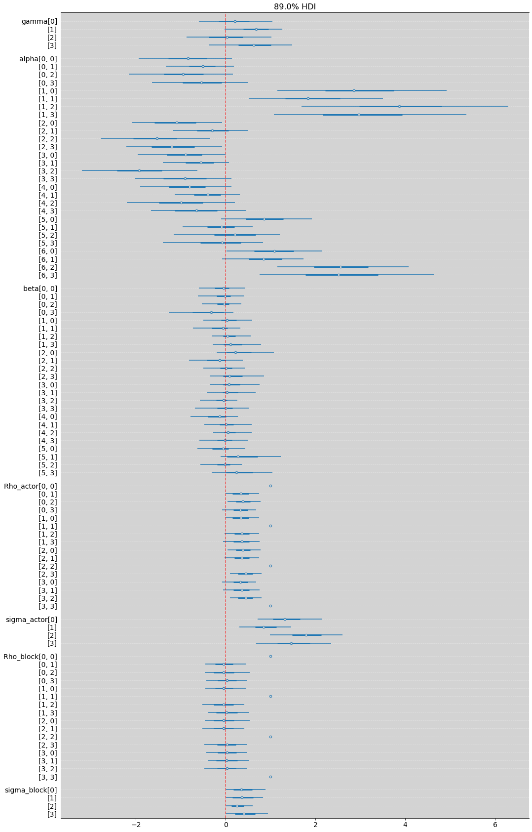
az.plot_forest(m_14_2, hdi_prob=0.89, combined=True, figsize=(17, 30))
plt.grid(axis='y', ls='--', color='white', alpha=0.3)
plt.axvline(x=0, color='red', ls='--', alpha=0.6)
plt.show()

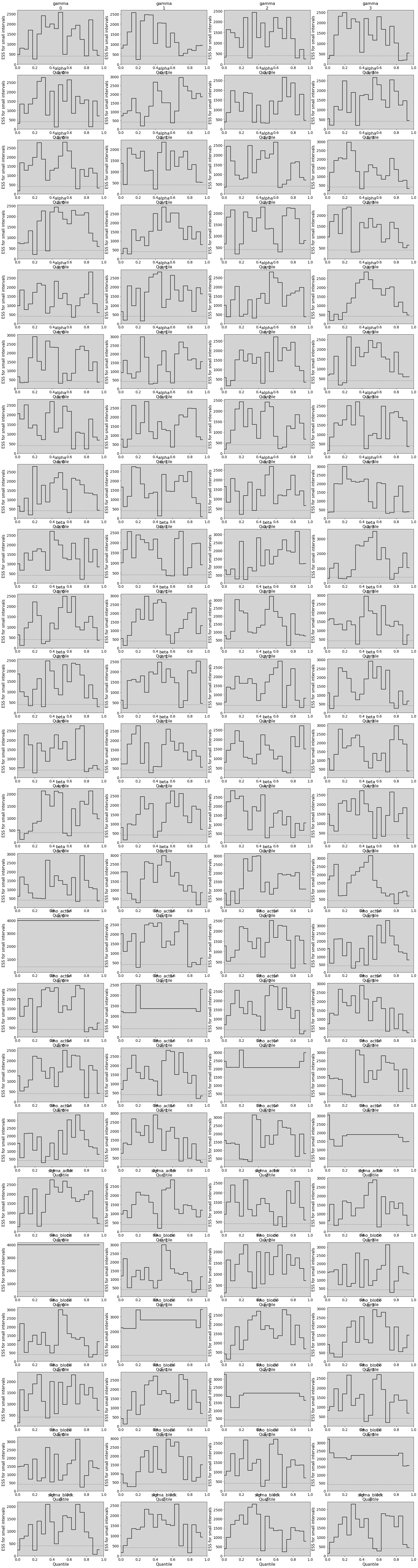
# Like trankplot in this book

az.rcParams['plot.max_subplots'] = 100

az.plot_ess(
    m_14_2, kind="local", drawstyle="steps-mid", color="k",
    linestyle="-", marker=None
)
plt.show()

R Code 14.19¶

# Undertanding Cholesky
rho_test = 0.3
R_test = np.matrix([[1, rho_test], [rho_test, 1]])
R_test

matrix([[1. , 0.3],
        [0.3, 1. ]])

# Cholesky decomposition
cholesky_matrix_L = np.linalg.cholesky(R_test)
cholesky_matrix_L

matrix([[1.       , 0.       ],
        [0.3      , 0.9539392]])

# Testing that R=LL^t
cholesky_matrix_L * np.transpose(cholesky_matrix_L)

matrix([[1. , 0.3],
        [0.3, 1. ]])

sample_uncorrelated_z_score = np.random.normal(0, 1, [2,200]) # ?
np.corrcoef(sample_uncorrelated_z_score)

array([[ 1.        , -0.15506489],
       [-0.15506489,  1.        ]])

How this model is works?¶

To understanding the chunck of code below.

    transformed parameters{
        matrix[qty_treatments, qty_chimpanzees] alpha;
        matrix[qty_treatments, qty_blocks] beta;
        
        alpha = (diag_pre_multiply(sigma_actor, L_Rho_actor) * z_actor)';
        beta = (diag_pre_multiply(sigma_block, L_Rho_block) * z_block)';   
    }

PS: $qty\_actor$ is equal to $qty\_chimpanzees$ for this example!

Firts, thinking about matrices dimensions:

To z’s ($z_{anything}$)

z_actor: $[qty\_treatment, qty\_actor]$
z_block: $[qty\_treatment, qty\_block]$

To sigmas ($\sigma$):

sigma_actor: $\sigma_{_{ACTOR}}[qty\_treatments]$
sigma_block: $\sigma_{_{BLOCK}}[qty\_treatments]$

To Rho’s ($\rho$):

L_Rho_actor: $\rho_{_{ACTOR}}[qty\_treatments \times qty\_treatments]$
L_Rho_block: $\rho_{_{BLOCK}}[qty\_treatments \times qty\_treatments]$

Now, understanding the stan functions:

The Stan function diag_pre_multiply works:

matrix diag_pre_multiply(vector v, matrix m)

Return the product of the diagonal matrix formed from the vector v and the matrix m, i.e., diag_matrix(v) * m.

The Stan function diag_matrix(v) works:

matrix diag_matrix(vector x)

The diagonal matrix with diagonal x.

For example: $x = \begin{bmatrix} 0.25 \\ 0.30 \\ 0.25 \\ 0.20 \end{bmatrix}$ then diag_matrix(x) is equal $\begin{bmatrix} 0.25 & 0 & 0 & 0 \\ 0 & 0.30 & 0 & 0 \\ 0 & 0 & 0.25 & 0 \\ 0 & 0 & 0 & 0.20 \end{bmatrix}$, this is a $[4 \times 4]$ matrix.

Finally, understanding dimensions for alpha and beta:

Then, this diag_pre_multiply(sigma_actor, L_Rho_actor) is:

diag_matrix(sigma_actor) $\times$ L_Rho_actor $[qty\_treatments \times qty\_treatments] \times [qty\_treatments \times qty\_treatments] = [qty\_treatments \times qty\_treatments]$

The complete calculations, have this dimension:

(diag_pre_multiply(sigma_actor, L_Rho_actor) * z_actor)

$[qty\_treatments \times qty\_treatments] \times [qty\_treatments \times qty\_chimpanzees] = [qty\_treatments \times qty\_chimpanzees]$

And to finish, transpose the matrix ( ’ ):

(diag_pre_multiply(sigma_actor, L_Rho_actor) * z_actor)'

$[qty\_chimpanzees \times qty\_treatments]$

Each of the index in matrix above, is a prior to alpha (or beta) in the model. Make the model with this structure is not need using the multi_normal(), like the previous model m_14_2.

model = """
    data {
        int N;
        int qty_chimpanzees;
        int qty_blocks;
        int qty_treatments;
        
        array[N] int pulled_left;
        array[N] int actor;
        array[N] int block;
        array[N] int treatment;
    }
    
    parameters{
        vector[qty_treatments] gamma;
        
        matrix[qty_treatments, qty_chimpanzees] z_actor;
        cholesky_factor_corr[qty_treatments] L_Rho_actor;
        vector<lower=0>[qty_treatments] sigma_actor;
        
        matrix[qty_treatments, qty_blocks] z_block;
        cholesky_factor_corr[qty_treatments] L_Rho_block;
        vector<lower=0>[qty_treatments] sigma_block;
    }
    
    transformed parameters{
        matrix[qty_chimpanzees, qty_treatments] alpha;
        matrix[qty_blocks, qty_treatments] beta;
        
        alpha = (diag_pre_multiply(sigma_actor, L_Rho_actor) * z_actor)';  // matrix[qty_actors, qty_treatments]
        beta = (diag_pre_multiply(sigma_block, L_Rho_block) * z_block)';   // Above explanations about this part
    }
    
    model {
        vector[N] p;
    
        // Adaptative Priors - Non-centered
        gamma ~ normal(0, 1);
    
        to_vector(z_actor) ~ normal(0, 1);
        L_Rho_actor ~ lkj_corr_cholesky(2);
        sigma_actor ~ exponential(1);
        
        to_vector(z_block) ~ normal(0, 1);
        L_Rho_block ~ lkj_corr_cholesky(2);
        sigma_block ~ exponential(1);
        
        // Linear model
        for (i in 1:N){
            p[i] = gamma[ treatment[i] ] + alpha[ actor[i], treatment[i] ] + beta[ block[i], treatment[i] ];
            p[i] = inv_logit(p[i]);  // Link function
        }
    
    
        // Likelihood
        pulled_left ~ binomial(1, p);
    }
 
"""


dat_list = df[['pulled_left', 'actor', 'block', 'treatment']].to_dict('list')
dat_list['N'] = len(df)
dat_list['qty_chimpanzees'] = len(df['actor'].unique())
dat_list['qty_blocks'] = len(df['block'].unique())
dat_list['qty_treatments'] = len(df['treatment'].unique())

posteriori = stan.build(model, data=dat_list)
samples = posteriori.sample(num_chains=4, num_samples=1000)

 m_14_3 = az.from_pystan(
     posterior=samples,
     posterior_model=posteriori,
     observed_data=dat_list.keys()
 )

print(az.summary(m_14_3, hdi_prob=0.89).to_string())

/home/rodolpho/Projects/bayesian/BAYES/lib/python3.8/site-packages/arviz/stats/diagnostics.py:592: RuntimeWarning: invalid value encountered in double_scalars
  (between_chain_variance / within_chain_variance + num_samples - 1) / (num_samples)
/home/rodolpho/Projects/bayesian/BAYES/lib/python3.8/site-packages/arviz/stats/diagnostics.py:592: RuntimeWarning: invalid value encountered in double_scalars
  (between_chain_variance / within_chain_variance + num_samples - 1) / (num_samples)
/home/rodolpho/Projects/bayesian/BAYES/lib/python3.8/site-packages/arviz/stats/diagnostics.py:592: RuntimeWarning: invalid value encountered in double_scalars
  (between_chain_variance / within_chain_variance + num_samples - 1) / (num_samples)
/home/rodolpho/Projects/bayesian/BAYES/lib/python3.8/site-packages/arviz/stats/diagnostics.py:592: RuntimeWarning: invalid value encountered in double_scalars
  (between_chain_variance / within_chain_variance + num_samples - 1) / (num_samples)
/home/rodolpho/Projects/bayesian/BAYES/lib/python3.8/site-packages/arviz/stats/diagnostics.py:592: RuntimeWarning: invalid value encountered in double_scalars
  (between_chain_variance / within_chain_variance + num_samples - 1) / (num_samples)
/home/rodolpho/Projects/bayesian/BAYES/lib/python3.8/site-packages/arviz/stats/diagnostics.py:592: RuntimeWarning: invalid value encountered in double_scalars
  (between_chain_variance / within_chain_variance + num_samples - 1) / (num_samples)

                    mean     sd  hdi_5.5%  hdi_94.5%  mcse_mean  mcse_sd  ess_bulk  ess_tail  r_hat
gamma[0]           0.214  0.484    -0.542      1.008      0.010    0.007    2269.0    2705.0    1.0
gamma[1]           0.647  0.407     0.032      1.306      0.008    0.006    2707.0    2436.0    1.0
gamma[2]          -0.009  0.585    -0.864      0.968      0.010    0.008    3341.0    2985.0    1.0
gamma[3]           0.671  0.548    -0.172      1.536      0.009    0.007    3377.0    2959.0    1.0
z_actor[0, 0]     -0.658  0.470    -1.387      0.108      0.009    0.006    2676.0    2969.0    1.0
z_actor[0, 1]      2.352  0.703     1.268      3.497      0.012    0.008    3693.0    3535.0    1.0
z_actor[0, 2]     -0.860  0.497    -1.641     -0.076      0.010    0.007    2512.0    2995.0    1.0
z_actor[0, 3]     -0.736  0.493    -1.505      0.048      0.010    0.007    2441.0    2824.0    1.0
z_actor[0, 4]     -0.643  0.468    -1.395      0.070      0.009    0.006    2762.0    3063.0    1.0
z_actor[0, 5]      0.594  0.481    -0.177      1.337      0.009    0.006    2830.0    3060.0    1.0
z_actor[0, 6]      0.959  0.565     0.054      1.810      0.011    0.008    2879.0    2906.0    1.0
z_actor[1, 0]     -0.375  0.667    -1.421      0.704      0.010    0.009    4046.0    3209.0    1.0
z_actor[1, 1]      1.410  0.923    -0.070      2.856      0.015    0.011    3558.0    3111.0    1.0
z_actor[1, 2]     -0.040  0.679    -1.112      1.050      0.012    0.009    3032.0    2925.0    1.0
z_actor[1, 3]     -0.438  0.688    -1.586      0.616      0.012    0.009    3536.0    3026.0    1.0
z_actor[1, 4]     -0.200  0.653    -1.248      0.814      0.011    0.009    3465.0    3298.0    1.0
z_actor[1, 5]     -0.360  0.664    -1.430      0.663      0.010    0.009    4207.0    3114.0    1.0
z_actor[1, 6]      0.774  0.799    -0.428      2.097      0.014    0.010    3292.0    3337.0    1.0
z_actor[2, 0]     -0.095  0.658    -1.202      0.861      0.010    0.011    4251.0    3045.0    1.0
z_actor[2, 1]      0.854  0.954    -0.696      2.299      0.014    0.011    4868.0    3715.0    1.0
z_actor[2, 2]     -0.512  0.685    -1.579      0.576      0.011    0.009    3935.0    2990.0    1.0
z_actor[2, 3]     -0.650  0.685    -1.766      0.410      0.011    0.008    3896.0    3334.0    1.0
z_actor[2, 4]     -0.172  0.652    -1.186      0.869      0.010    0.009    4222.0    2968.0    1.0
z_actor[2, 5]     -0.102  0.669    -1.088      0.987      0.011    0.009    3832.0    3130.0    1.0
z_actor[2, 6]      0.988  0.853    -0.343      2.307      0.014    0.010    3600.0    3031.0    1.0
z_actor[3, 0]      0.071  0.750    -1.127      1.247      0.010    0.011    5689.0    2879.0    1.0
z_actor[3, 1]      0.466  0.929    -1.026      1.906      0.011    0.013    7144.0    3451.0    1.0
z_actor[3, 2]     -0.412  0.766    -1.645      0.780      0.011    0.010    5330.0    3191.0    1.0
z_actor[3, 3]      0.015  0.768    -1.291      1.159      0.010    0.013    5528.0    2981.0    1.0
z_actor[3, 4]     -0.088  0.715    -1.262      0.998      0.010    0.011    5285.0    3284.0    1.0
z_actor[3, 5]     -0.322  0.753    -1.551      0.835      0.010    0.010    5436.0    3206.0    1.0
z_actor[3, 6]      0.831  0.928    -0.635      2.293      0.011    0.011    6855.0    2990.0    1.0
L_Rho_actor[0, 0]  1.000  0.000     1.000      1.000      0.000    0.000    4000.0    4000.0    NaN
L_Rho_actor[0, 1]  0.000  0.000     0.000      0.000      0.000    0.000    4000.0    4000.0    NaN
L_Rho_actor[0, 2]  0.000  0.000     0.000      0.000      0.000    0.000    4000.0    4000.0    NaN
L_Rho_actor[0, 3]  0.000  0.000     0.000      0.000      0.000    0.000    4000.0    4000.0    NaN
L_Rho_actor[1, 0]  0.431  0.276     0.007      0.855      0.005    0.004    2884.0    3014.0    1.0
L_Rho_actor[1, 1]  0.848  0.141     0.650      1.000      0.003    0.002    2922.0    3014.0    1.0
L_Rho_actor[1, 2]  0.000  0.000     0.000      0.000      0.000    0.000    4000.0    4000.0    NaN
L_Rho_actor[1, 3]  0.000  0.000     0.000      0.000      0.000    0.000    4000.0    4000.0    NaN
L_Rho_actor[2, 0]  0.532  0.248     0.164      0.903      0.004    0.003    3145.0    3045.0    1.0
L_Rho_actor[2, 1]  0.282  0.307    -0.181      0.784      0.006    0.005    2295.0    3168.0    1.0
L_Rho_actor[2, 2]  0.670  0.179     0.398      0.961      0.003    0.002    2869.0    3066.0    1.0
L_Rho_actor[2, 3]  0.000  0.000     0.000      0.000      0.000    0.000    4000.0    4000.0    NaN
L_Rho_actor[3, 0]  0.452  0.262     0.050      0.849      0.005    0.004    2657.0    3037.0    1.0
L_Rho_actor[3, 1]  0.274  0.315    -0.185      0.806      0.006    0.004    2731.0    3051.0    1.0
L_Rho_actor[3, 2]  0.293  0.317    -0.204      0.790      0.006    0.004    2498.0    2774.0    1.0
L_Rho_actor[3, 3]  0.579  0.180     0.291      0.865      0.003    0.002    2690.0    3154.0    1.0
sigma_actor[0]     1.383  0.489     0.664      2.025      0.010    0.007    2353.0    3000.0    1.0
sigma_actor[1]     0.901  0.404     0.296      1.434      0.007    0.005    2969.0    2671.0    1.0
sigma_actor[2]     1.845  0.592     0.931      2.608      0.011    0.009    3250.0    2401.0    1.0
sigma_actor[3]     1.568  0.582     0.669      2.312      0.011    0.008    3144.0    2650.0    1.0
z_block[0, 0]     -0.279  0.844    -1.581      1.139      0.012    0.012    5021.0    2942.0    1.0
z_block[0, 1]      0.115  0.834    -1.279      1.396      0.011    0.013    5926.0    3115.0    1.0
z_block[0, 2]      0.664  0.865    -0.682      2.039      0.012    0.010    4964.0    3108.0    1.0
z_block[0, 3]      0.268  0.840    -1.125      1.535      0.011    0.014    5965.0    3090.0    1.0
z_block[0, 4]     -0.429  0.844    -1.837      0.803      0.012    0.012    5334.0    3088.0    1.0
z_block[0, 5]     -0.256  0.885    -1.622      1.198      0.012    0.013    5104.0    3190.0    1.0
z_block[1, 0]     -0.139  0.877    -1.574      1.206      0.012    0.014    5667.0    3063.0    1.0
z_block[1, 1]     -0.252  0.820    -1.567      1.065      0.010    0.014    6141.0    2950.0    1.0
z_block[1, 2]     -0.402  0.841    -1.747      0.953      0.011    0.012    5565.0    3300.0    1.0
z_block[1, 3]      0.240  0.853    -1.050      1.629      0.011    0.013    6536.0    3148.0    1.0
z_block[1, 4]      0.035  0.803    -1.282      1.268      0.010    0.012    6050.0    3079.0    1.0
z_block[1, 5]      0.795  0.882    -0.606      2.209      0.013    0.011    4431.0    3202.0    1.0
z_block[2, 0]     -0.128  0.942    -1.655      1.339      0.012    0.015    5812.0    3369.0    1.0
z_block[2, 1]      0.174  0.962    -1.432      1.656      0.011    0.016    7222.0    3020.0    1.0
z_block[2, 2]      0.019  0.938    -1.537      1.437      0.011    0.018    7040.0    2325.0    1.0
z_block[2, 3]     -0.268  0.893    -1.619      1.242      0.011    0.014    7031.0    3159.0    1.0
z_block[2, 4]      0.235  0.932    -1.228      1.746      0.011    0.015    7393.0    3028.0    1.0
z_block[2, 5]     -0.069  0.926    -1.558      1.387      0.012    0.016    6284.0    3006.0    1.0
z_block[3, 0]     -0.614  0.961    -2.149      0.915      0.012    0.012    6496.0    3194.0    1.0
z_block[3, 1]      0.258  0.907    -1.227      1.666      0.011    0.015    6812.0    2742.0    1.0
z_block[3, 2]      0.239  0.900    -1.211      1.650      0.011    0.014    6636.0    3177.0    1.0
z_block[3, 3]     -0.012  0.933    -1.528      1.462      0.011    0.016    6781.0    2974.0    1.0
z_block[3, 4]     -0.061  0.913    -1.435      1.453      0.011    0.016    7351.0    3078.0    1.0
z_block[3, 5]      0.454  0.930    -1.027      1.931      0.011    0.014    6617.0    2932.0    1.0
L_Rho_block[0, 0]  1.000  0.000     1.000      1.000      0.000    0.000    4000.0    4000.0    NaN
L_Rho_block[0, 1]  0.000  0.000     0.000      0.000      0.000    0.000    4000.0    4000.0    NaN
L_Rho_block[0, 2]  0.000  0.000     0.000      0.000      0.000    0.000    4000.0    4000.0    NaN
L_Rho_block[0, 3]  0.000  0.000     0.000      0.000      0.000    0.000    4000.0    4000.0    NaN
L_Rho_block[1, 0] -0.062  0.374    -0.623      0.574      0.005    0.006    4592.0    3122.0    1.0
L_Rho_block[1, 1]  0.920  0.097     0.794      1.000      0.002    0.001    2692.0    3089.0    1.0
L_Rho_block[1, 2]  0.000  0.000     0.000      0.000      0.000    0.000    4000.0    4000.0    NaN
L_Rho_block[1, 3]  0.000  0.000     0.000      0.000      0.000    0.000    4000.0    4000.0    NaN
L_Rho_block[2, 0] -0.020  0.378    -0.649      0.557      0.004    0.007    7142.0    2844.0    1.0
L_Rho_block[2, 1] -0.035  0.365    -0.602      0.562      0.004    0.006    7624.0    3040.0    1.0
L_Rho_block[2, 2]  0.839  0.135     0.655      1.000      0.003    0.002    1757.0    2150.0    1.0
L_Rho_block[2, 3]  0.000  0.000     0.000      0.000      0.000    0.000    4000.0    4000.0    NaN
L_Rho_block[3, 0]  0.045  0.379    -0.552      0.663      0.005    0.006    5021.0    3052.0    1.0
L_Rho_block[3, 1]  0.056  0.373    -0.487      0.709      0.005    0.006    4887.0    3093.0    1.0
L_Rho_block[3, 2]  0.012  0.373    -0.572      0.627      0.005    0.006    4738.0    2872.0    1.0
L_Rho_block[3, 3]  0.739  0.166     0.508      0.986      0.004    0.003    2069.0    2228.0    1.0
sigma_block[0]     0.400  0.321     0.000      0.796      0.006    0.004    2252.0    2283.0    1.0
sigma_block[1]     0.445  0.344     0.000      0.892      0.007    0.005    1967.0    2353.0    1.0
sigma_block[2]     0.303  0.268     0.000      0.627      0.004    0.003    3314.0    2291.0    1.0
sigma_block[3]     0.473  0.375     0.000      0.938      0.007    0.005    1971.0    2057.0    1.0
alpha[0, 0]       -0.844  0.609    -1.798      0.138      0.011    0.008    3018.0    3108.0    1.0
alpha[0, 1]       -0.511  0.488    -1.332      0.210      0.008    0.006    3697.0    3196.0    1.0
alpha[0, 2]       -0.968  0.724    -2.073      0.196      0.012    0.009    3837.0    3287.0    1.0
alpha[0, 3]       -0.573  0.659    -1.688      0.384      0.011    0.008    3787.0    3380.0    1.0
alpha[1, 0]        3.152  1.250     1.301      4.881      0.020    0.015    4111.0    3012.0    1.0
alpha[1, 1]        2.005  0.994     0.487      3.404      0.017    0.012    3564.0    2907.0    1.0
alpha[1, 2]        4.309  1.662     1.993      6.688      0.026    0.019    4333.0    3691.0    1.0
alpha[1, 3]        3.406  1.531     1.284      5.719      0.024    0.018    4224.0    3729.0    1.0
alpha[2, 0]       -1.107  0.627    -2.048     -0.059      0.012    0.008    2984.0    2985.0    1.0
alpha[2, 1]       -0.326  0.475    -1.061      0.424      0.008    0.006    3701.0    3368.0    1.0
alpha[2, 2]       -1.537  0.758    -2.752     -0.397      0.012    0.009    3838.0    3581.0    1.0
alpha[2, 3]       -1.298  0.660    -2.315     -0.265      0.011    0.008    3689.0    3640.0    1.0
alpha[3, 0]       -0.937  0.609    -1.988     -0.034      0.011    0.008    2847.0    2833.0    1.0
alpha[3, 1]       -0.580  0.489    -1.425      0.103      0.008    0.006    3921.0    3536.0    1.0
alpha[3, 2]       -1.833  0.810    -3.070     -0.571      0.013    0.009    3685.0    3422.0    1.0
alpha[3, 3]       -0.976  0.655    -1.992      0.053      0.010    0.007    3970.0    3603.0    1.0
alpha[4, 0]       -0.830  0.606    -1.803      0.092      0.011    0.008    2947.0    3191.0    1.0
alpha[4, 1]       -0.376  0.476    -1.180      0.332      0.008    0.006    3636.0    3293.0    1.0
alpha[4, 2]       -0.970  0.726    -2.106      0.157      0.012    0.009    3644.0    3421.0    1.0
alpha[4, 3]       -0.701  0.649    -1.760      0.301      0.010    0.008    4094.0    3235.0    1.0
alpha[5, 0]        0.781  0.638    -0.226      1.775      0.013    0.009    2588.0    3109.0    1.0
alpha[5, 1]       -0.047  0.489    -0.838      0.713      0.008    0.006    3884.0    2572.0    1.0
alpha[5, 2]        0.247  0.705    -0.802      1.415      0.012    0.009    3467.0    3059.0    1.0
alpha[5, 3]       -0.099  0.654    -1.140      0.903      0.011    0.008    3396.0    3452.0    1.0
alpha[6, 0]        1.206  0.661     0.164      2.255      0.012    0.009    2952.0    3040.0    1.0
alpha[6, 1]        0.923  0.590    -0.008      1.821      0.010    0.007    3706.0    3387.0    1.0
alpha[6, 2]        2.644  0.948     1.114      4.069      0.015    0.010    4093.0    3203.0    1.0
alpha[6, 3]        2.583  1.238     0.819      4.327      0.021    0.015    3962.0    2851.0    1.0
beta[0, 0]        -0.128  0.347    -0.694      0.366      0.005    0.005    4443.0    3501.0    1.0
beta[0, 1]        -0.052  0.356    -0.625      0.522      0.005    0.004    5006.0    3834.0    1.0
beta[0, 2]        -0.051  0.296    -0.509      0.410      0.005    0.004    3767.0    3333.0    1.0
beta[0, 3]        -0.410  0.502    -1.230      0.177      0.009    0.006    2840.0    3496.0    1.0
beta[1, 0]         0.055  0.337    -0.446      0.622      0.005    0.005    4781.0    3152.0    1.0
beta[1, 1]        -0.133  0.354    -0.723      0.371      0.005    0.004    4166.0    3478.0    1.0
beta[1, 2]         0.083  0.319    -0.308      0.653      0.005    0.004    4656.0    3749.0    1.0
beta[1, 3]         0.170  0.382    -0.395      0.780      0.006    0.005    3841.0    3438.0    1.0
beta[2, 0]         0.317  0.425    -0.208      0.992      0.007    0.005    3416.0    3690.0    1.0
beta[2, 1]        -0.234  0.384    -0.862      0.274      0.006    0.004    4393.0    3765.0    1.0
beta[2, 2]         0.005  0.301    -0.433      0.478      0.005    0.004    4467.0    3665.0    1.0
beta[2, 3]         0.160  0.395    -0.419      0.786      0.007    0.005    3436.0    3374.0    1.0
beta[3, 0]         0.132  0.363    -0.347      0.765      0.006    0.005    4384.0    3346.0    1.0
beta[3, 1]         0.121  0.373    -0.460      0.688      0.006    0.005    4625.0    3475.0    1.0
beta[3, 2]        -0.118  0.299    -0.600      0.284      0.005    0.004    3625.0    3715.0    1.0
beta[3, 3]         0.020  0.397    -0.618      0.661      0.006    0.005    4497.0    3784.0    1.0
beta[4, 0]        -0.206  0.380    -0.852      0.282      0.006    0.005    3851.0    3106.0    1.0
beta[4, 1]         0.049  0.350    -0.496      0.606      0.005    0.004    4743.0    3521.0    1.0
beta[4, 2]         0.111  0.315    -0.276      0.632      0.005    0.004    4500.0    3759.0    1.0
beta[4, 3]        -0.027  0.363    -0.617      0.522      0.006    0.005    4160.0    3394.0    1.0
beta[5, 0]        -0.129  0.364    -0.757      0.365      0.005    0.005    4804.0    3337.0    1.0
beta[5, 1]         0.436  0.499    -0.158      1.206      0.010    0.007    2438.0    3590.0    1.0
beta[5, 2]        -0.047  0.299    -0.479      0.404      0.005    0.003    3962.0    3423.0    1.0
beta[5, 3]         0.328  0.482    -0.272      1.100      0.008    0.006    3374.0    3766.0    1.0

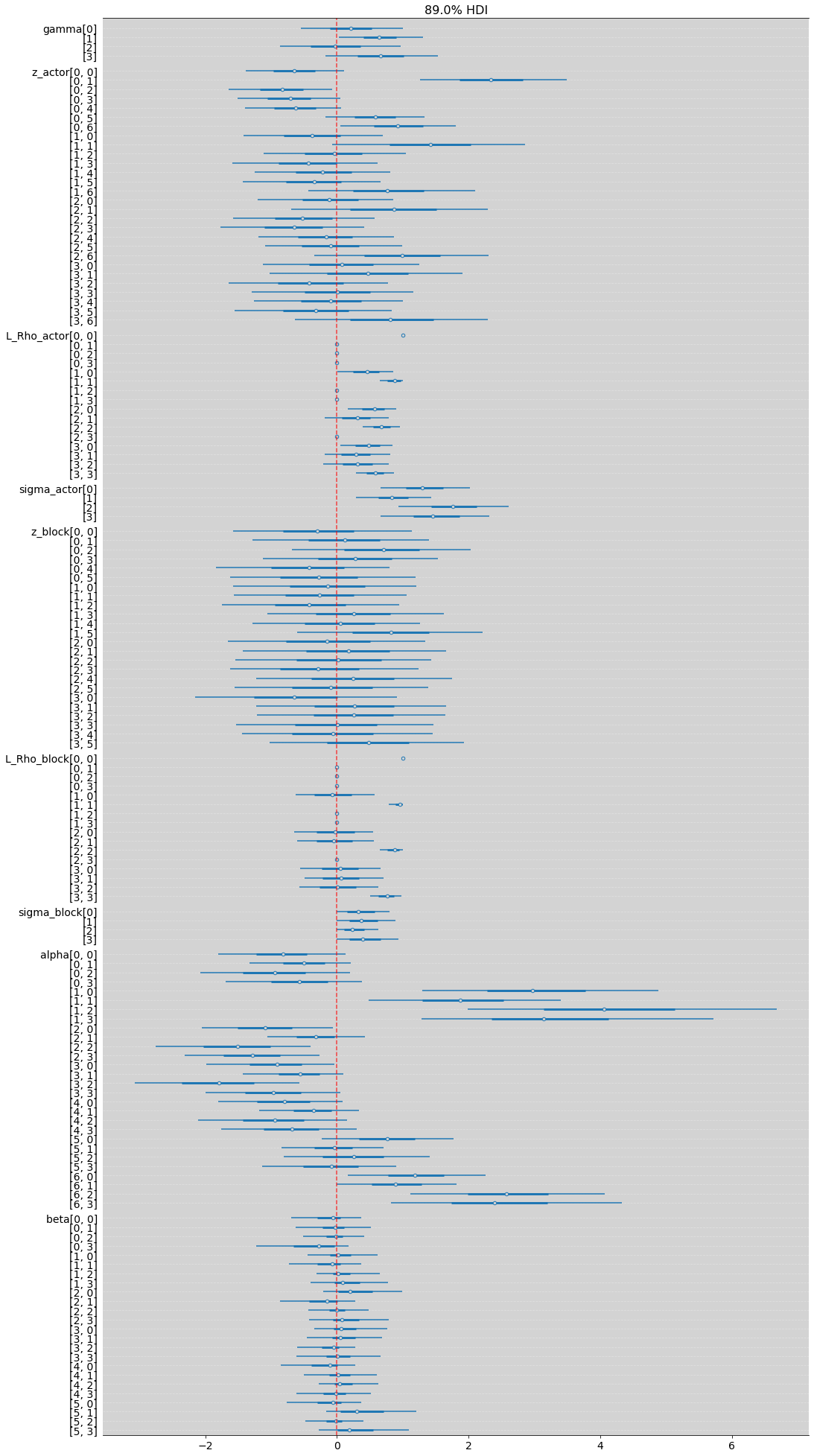
az.plot_forest(m_14_3, combined=True, hdi_prob=0.89, figsize=(17, 35))

plt.axvline(x=0, color='red', ls='--', alpha=0.7)
plt.grid(axis='y', color='white', ls='--', alpha=0.3)

plt.show()

R Code 14.20¶

import matplotlib.pyplot as plt
from importlib import reload
plt=reload(plt)

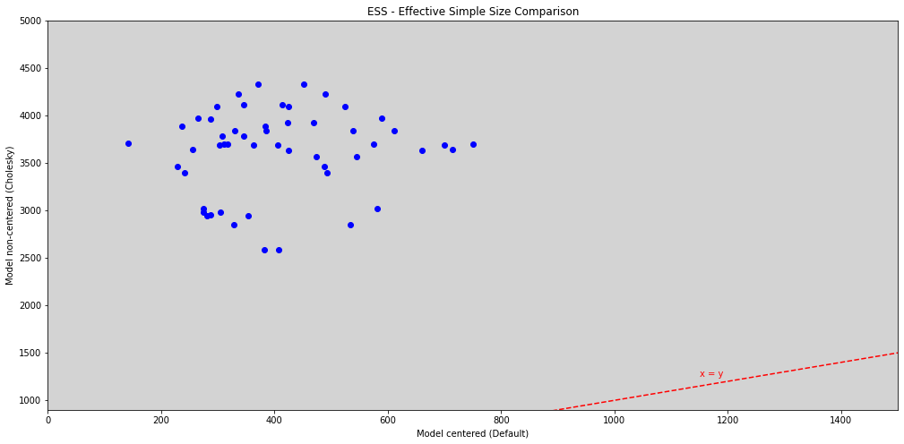
alpha_ess_14_3 = az.ess(m_14_3, var_names=["alpha", "beta"]).alpha.values.flatten()
beta_ess_14_3 = az.ess(m_14_3, var_names=["alpha", "beta"]).alpha.values.flatten()

alpha_ess_14_2 = az.ess(m_14_2, var_names=["alpha", "beta"]).alpha.values.flatten()
beta_ess_14_2 = az.ess(m_14_2, var_names=["alpha", "beta"]).beta.values.flatten()

plt.figure(figsize=(17, 8))

plt.scatter(alpha_ess_14_2, alpha_ess_14_3, c='b')
plt.scatter(beta_ess_14_2, beta_ess_14_3[:24], c='b')

plt.plot([0, 5000], [0, 5000], ls='--', c='red')
plt.text(1150, 1250, 'x = y', color='red')

plt.ylim(900, 5000)
plt.xlim(0, 1500)

plt.title('ESS - Effective Simple Size Comparison')
plt.xlabel('Model centered (Default)')
plt.ylabel('Model non-centered (Cholesky)')

plt.show()

R Code 14.21¶

az.summary(m_14_3, var_names=['sigma_actor', 'sigma_block'], hdi_prob=0.89)

	mean	sd	hdi_5.5%	hdi_94.5%	mcse_mean	mcse_sd	ess_bulk	ess_tail	r_hat
sigma_actor[0]	1.383	0.489	0.664	2.025	0.010	0.007	2353.0	3000.0	1.0
sigma_actor[1]	0.901	0.404	0.296	1.434	0.007	0.005	2969.0	2671.0	1.0
sigma_actor[2]	1.845	0.592	0.931	2.608	0.011	0.009	3250.0	2401.0	1.0
sigma_actor[3]	1.568	0.582	0.669	2.312	0.011	0.008	3144.0	2650.0	1.0
sigma_block[0]	0.400	0.321	0.000	0.796	0.006	0.004	2252.0	2283.0	1.0
sigma_block[1]	0.445	0.344	0.000	0.892	0.007	0.005	1967.0	2353.0	1.0
sigma_block[2]	0.303	0.268	0.000	0.627	0.004	0.003	3314.0	2291.0	1.0
sigma_block[3]	0.473	0.375	0.000	0.938	0.007	0.005	1971.0	2057.0	1.0

R Code 14.22¶

# Like R Code 11.17
# ==================

TODO = """
plt.figure(figsize=(18, 6))

plt.ylim(0, 1.3)
plt.xlim(0, 7)
plt.axhline(y=1, ls='-', c='black')
plt.axhline(y=0.5, ls='--', c='black')


for i in range(7):
    plt.axvline(x=i+1, c='black')
    plt.text(x=i + 0.25, y=1.1, s=f'Actor {i + 1}', size=20)
    
    alpha_chimp = az.extract(samples_chimpanzees.posterior.alpha.sel(alpha_dim_0=i)).alpha.values
    
    RN = inv_logit(alpha_chimp + az.extract(samples_chimpanzees.posterior.beta.sel(beta_dim_0=0)).beta.values)
    LN = inv_logit(alpha_chimp + az.extract(samples_chimpanzees.posterior.beta.sel(beta_dim_0=1)).beta.values)
    RP = inv_logit(alpha_chimp + az.extract(samples_chimpanzees.posterior.beta.sel(beta_dim_0=2)).beta.values)
    LP = inv_logit(alpha_chimp + az.extract(samples_chimpanzees.posterior.beta.sel(beta_dim_0=3)).beta.values)
    
    # To R/N and R/P
    # ===============
    if not i == 1:
        plt.plot([0.2 + i, 0.8 + i], [RN.mean(), RP.mean()], color='black')
    
    # Plot hdi compatibility interval
    RN_hdi_min, RN_hdi_max = az.hdi(RN, hdi_prob=0.89)
    RP_hdi_min, RP_hdi_max = az.hdi(RP, hdi_prob=0.89)
    plt.plot([0.2 + i, 0.2 + i], [RN_hdi_min, RN_hdi_max], c='black')
    plt.plot([0.8 + i, 0.8 + i], [RP_hdi_min, RP_hdi_max], c='black')
    
    # Plot points
    plt.plot(0.2 + i, RN.mean(), 'o', markerfacecolor='white', color='black')
    plt.plot(0.8 + i, RP.mean(), 'o', markerfacecolor='black', color='white')
    
    # To L/N and L/P
    # ===============
    if not i == 1:
        plt.plot([0.3 + i, 0.9 + i], [LN.mean(), LP.mean()], color='black', linewidth=3)

    # Plot hdi compatibility interval
    LN_hdi_min, LN_hdi_max = az.hdi(LN, hdi_prob=0.89)
    LP_hdi_min, LP_hdi_max = az.hdi(LP, hdi_prob=0.89)
    plt.plot([0.3 + i, 0.3 + i], [LN_hdi_min, LN_hdi_max], c='black')
    plt.plot([0.9 + i, 0.9 + i], [LP_hdi_min, LP_hdi_max], c='black')

    plt.plot(0.3 + i, LN.mean(), 'o', markerfacecolor='white', color='black')
    plt.plot(0.9 + i, LP.mean(), 'o', markerfacecolor='black', color='white')
    
    # Labels for only first points
    if i == 0:
        plt.text(x=0.08, y=RN.mean() - 0.08, s='R/N')
        plt.text(x=0.68, y=RP.mean() - 0.08, s='R/P')
        plt.text(x=0.17, y=LN.mean() + 0.08, s='L/N')
        plt.text(x=0.77, y=LP.mean() + 0.08, s='L/P')
    
plt.title('Posterior Predictions')
plt.ylabel('Proportion left lever')
plt.yticks([0, 0.5, 1], [0, 0.5, 1])
plt.xticks([])

plt.show()
"""

# TODO: Rebuild to this example. 

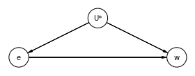
14.3 Instrumental and Causal Designs¶

The variable $^*U$ is an unobserved.

dag_14_3_1 = CausalGraphicalModel(
    nodes=['e', 'U*', 'w'],
    edges=[
        ('U*', 'e'),
        ('U*', 'w'),
        ('e', 'w')
    ],
)

# Drawing the DAG
pgm = daft.PGM()
coordinates = {
    "U*": (2, 1),
    "e": (0, 0),
    "w": (4, 0),
}
for node in dag_14_3_1.dag.nodes:
    pgm.add_node(node, node, *coordinates[node])
for edge in dag_14_3_1.dag.edges:
    pgm.add_edge(*edge)
pgm.render()

plt.show()

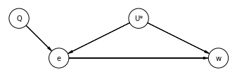
Now, we add Instrumental Variable Q:

dag_14_3_1 = CausalGraphicalModel(
    nodes=['e', 'U*', 'w', 'Q'],
    edges=[
        ('U*', 'e'),
        ('U*', 'w'),
        ('e', 'w'),
        ('Q', 'e')
    ],
)

# Drawing the DAG
pgm = daft.PGM()
coordinates = {
    "U*": (3, 1),
    "e": (1, 0),
    "w": (5, 0),
    "Q": (0, 1),
}
for node in dag_14_3_1.dag.nodes:
    pgm.add_node(node, node, *coordinates[node])
for edge in dag_14_3_1.dag.edges:
    pgm.add_edge(*edge)
pgm.render()

plt.show()

R Code 14.23¶

def standartize(data, get_parameters=False):
    mean = np.mean(data)
    std = np.std(data)
    
    if not get_parameters:
        return list((data - mean)/std)
    else:
        return list((data - mean)/std), mean, std

N = 500

U_sim = np.random.normal(0, 1, N)
Q_sim = np.random.choice([1,2,3,4], size=N, replace=True)

E_sim = np.random.normal(U_sim + Q_sim, 1, N)  # E is influencied by U and Q
W_sim = np.random.normal(U_sim + 0*E_sim, 1, N)  # W is influencied only by U, not by E

dat_sim = pd.DataFrame({
    'W': standartize(W_sim),
    'E': standartize(E_sim),
    'Q': standartize(Q_sim)
})

dat_sim

	W	E	Q
0	0.458919	-1.050410	-1.412495
1	0.367655	0.827180	1.390074
2	-0.058669	0.095503	0.455884
3	0.139368	1.715983	0.455884
4	1.289500	1.171285	0.455884
...	...	...	...
495	-1.661304	0.222796	0.455884
496	0.078534	0.363780	0.455884
497	-0.341889	-1.104266	-1.412495
498	0.326049	-1.023097	-0.478305
499	2.156961	2.760130	1.390074

500 rows × 3 columns

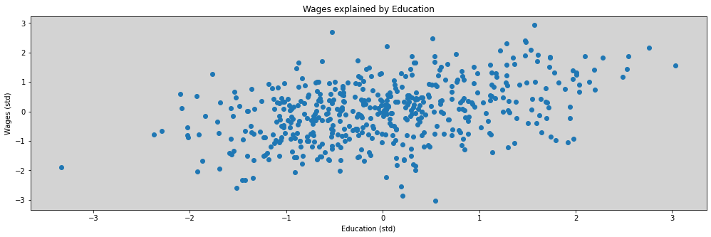
plt.figure(figsize=(17,5))

plt.plot(dat_sim.E, dat_sim.W, 'o')

plt.title('Wages explained by Education')
plt.xlabel('Education (std)')
plt.ylabel('Wages (std)')

plt.show()

model = """
    data {
        int N;
        array[N] real W;
        array[N] real E;
    }
    
    parameters {
        real aW;
        real bEW;
        real<lower=0> sigma;
    }
    
    model {
        array[N] real mu;
        
        aW ~ normal(0, 0.2);
        bEW ~ normal(0, 0.5);
        
        sigma ~ exponential(1);
        
        for (i in 1:N){
            mu[i] = aW + bEW*E[i];
        }
        
        W ~ normal(mu, sigma);
    }

"""

dat_list = {
    'N': len(dat_sim),
    'W': dat_sim.W.values,
    'E': dat_sim.E.values,
}

posteriori = stan.build(model, data=dat_list)
samples = posteriori.sample(num_chains=4, num_samples=1000)

model_14_4 = az.from_pystan(
    posterior=samples,
    posterior_model=posteriori,
    observed_data=dat_list.keys()
)

az.summary(model_14_4, hdi_prob=0.89)

	mean	sd	hdi_5.5%	hdi_94.5%	mcse_mean	mcse_sd	ess_bulk	ess_tail	r_hat
aW	-0.000	0.039	-0.066	0.057	0.001	0.001	3968.0	2939.0	1.0
bEW	0.413	0.040	0.349	0.479	0.001	0.000	3483.0	2369.0	1.0
sigma	0.912	0.030	0.867	0.961	0.000	0.000	4109.0	2633.0	1.0

R Code 14.25¶

model = """
    data {
        int N;
        array[N] real W;
        array[N] real E;
        array[N] real Q;
    }
    
    parameters {
        real aW;
        real bEW;
        real bQW;
        real<lower=0> sigma;
    }
    
    model {
        array[N] real mu;
        
        aW ~ normal(0, 0.2);
        bEW ~ normal(0, 0.5);
        bQW ~ normal(0, 0.5);
        
        sigma ~ exponential(1);
        
        for (i in 1:N){
            mu[i] = aW + bEW*E[i] + bQW*Q[i];
        }
        
        W ~ normal(mu, sigma);
    }

"""

dat_list = {
    'N': len(dat_sim),
    'W': dat_sim.W.values,
    'E': dat_sim.E.values,
    'Q': dat_sim.Q.values,
}

posteriori = stan.build(model, data=dat_list)
samples = posteriori.sample(num_chains=4, num_samples=1000)

model_14_5 = az.from_pystan(
    posterior=samples,
    posterior_model=posteriori,
    observed_data=dat_list.keys()
)

az.summary(model_14_5, hdi_prob=0.89)

	mean	sd	hdi_5.5%	hdi_94.5%	mcse_mean	mcse_sd	ess_bulk	ess_tail	r_hat
aW	-0.001	0.038	-0.062	0.060	0.001	0.001	3870.0	2998.0	1.0
bEW	0.633	0.050	0.556	0.712	0.001	0.001	3293.0	2912.0	1.0
bQW	-0.348	0.050	-0.421	-0.257	0.001	0.001	3419.0	2644.0	1.0
sigma	0.870	0.027	0.828	0.912	0.000	0.000	3886.0	3023.0	1.0

Include instrument variable $Q$, the bias increase. The bEW now is $0.6$ instead of $0.4$ from previous model. The results from the new model is terrible!

Now, we goes to use instrument variable correctly.

Let’s wirter four models, simples generative versions of the DAG’s.

The firt model for how wages $W$ are caused by education $E$ and the unobserverd confound $U$.

\[ W_i \sim Normal(\mu_{w,i}, \sigma_{w})\]

\[ \mu_{w, i} = \alpha_{w} + \beta_{EW}E_i + U_i \]

The second model, for education levels $E$ are caused by quarter of birth $Q$ and the same unobserved confound $U$.

\[ E_i \sim Normal(\mu_{E, i}, \sigma_E) \]

\[ \mu_{E, i} = \alpha_{E} + \beta_{QE}Q_i + U_i \]

The thirt model is for $Q$, that says that one-quarter of all people born in each quarter of the year.

\[ Q_i \sim Categorical([0.25, 0.25, 0.25, 0.25]) \]

Finally, the model says that the unobserved confound $U$ is normally distributed with mean standart gaussian.

\[ U_i \sim Normal(0, 1) \]

Now, we writer this generative model to statistical model, like multivariate normal distribution. Like this:

\[\begin{split}\begin{pmatrix} W_i \\ E_i \end{pmatrix} \sim MVNormal\begin{pmatrix} \begin{bmatrix} \mu_{w, i} \\ \mu_{E, i} \end{bmatrix}, S \end{pmatrix} \end{split}\]

	actor	recipient	block	trial	prosoc_left	chose_prosoc	pulled_left	treatment
0	1	NaN	1	2	0	1	0	1
1	1	NaN	1	4	0	0	1	1
2	1	NaN	1	6	1	0	0	2
3	1	NaN	1	8	0	1	0	1
4	1	NaN	1	10	1	1	1	2
5	1	NaN	1	12	1	1	1	2
6	1	NaN	2	14	1	0	0	2
7	1	NaN	2	16	1	0	0	2
8	1	NaN	2	18	0	1	0	1
9	1	NaN	2	20	0	1	0	1
10	1	NaN	2	22	0	0	1	1
11	1	NaN	2	24	1	0	0	2
12	1	NaN	3	26	0	0	1	1
13	1	NaN	3	28	1	1	1	2
14	1	NaN	3	30	0	1	0	1
15	1	NaN	3	32	1	1	1	2
16	1	NaN	3	34	1	0	0	2
17	1	NaN	3	36	0	1	0	1
18	1	NaN	4	38	1	1	1	2
19	1	NaN	4	40	0	0	1	1

	actor	recipient	condition	block	trial	prosoc_left	chose_prosoc	pulled_left	treatment
484	7	2.0	1	3	34	0	0	1	3
485	7	3.0	1	3	36	1	1	1	4
486	7	7.0	1	4	38	0	0	1	3
487	7	2.0	1	4	40	0	0	1	3
488	7	4.0	1	4	42	1	1	1	4
489	7	5.0	1	4	44	0	0	1	3
490	7	6.0	1	4	46	0	0	1	3
491	7	3.0	1	4	48	0	0	1	3
492	7	5.0	1	5	50	1	1	1	4
493	7	4.0	1	5	52	0	0	1	3
494	7	3.0	1	5	54	0	0	1	3
495	7	2.0	1	5	56	1	1	1	4
496	7	6.0	1	5	58	1	1	1	4
497	7	7.0	1	5	60	1	1	1	4
498	7	5.0	1	6	62	1	1	1	4
499	7	4.0	1	6	64	1	1	1	4
500	7	6.0	1	6	66	1	1	1	4
501	7	3.0	1	6	68	0	0	1	3
502	7	7.0	1	6	70	0	0	1	3
503	7	2.0	1	6	72	0	0	1	3

	actor	recipient	block	trial	prosoc_left	chose_prosoc	pulled_left	treatment
0	1	NaN	1	2	0	1	0	1
1	1	NaN	1	4	0	0	1	1
2	1	NaN	1	6	1	0	0	2
3	1	NaN	1	8	0	1	0	1
4	1	NaN	1	10	1	1	1	2
5	1	NaN	1	12	1	1	1	2
6	1	NaN	2	14	1	0	0	2
7	1	NaN	2	16	1	0	0	2
8	1	NaN	2	18	0	1	0	1
9	1	NaN	2	20	0	1	0	1
10	1	NaN	2	22	0	0	1	1
11	1	NaN	2	24	1	0	0	2
12	1	NaN	3	26	0	0	1	1
13	1	NaN	3	28	1	1	1	2
14	1	NaN	3	30	0	1	0	1
15	1	NaN	3	32	1	1	1	2
16	1	NaN	3	34	1	0	0	2
17	1	NaN	3	36	0	1	0	1
18	1	NaN	4	38	1	1	1	2
19	1	NaN	4	40	0	0	1	1

	actor	recipient	condition	block	trial	prosoc_left	chose_prosoc	pulled_left	treatment
484	7	2.0	1	3	34	0	0	1	3
485	7	3.0	1	3	36	1	1	1	4
486	7	7.0	1	4	38	0	0	1	3
487	7	2.0	1	4	40	0	0	1	3
488	7	4.0	1	4	42	1	1	1	4
489	7	5.0	1	4	44	0	0	1	3
490	7	6.0	1	4	46	0	0	1	3
491	7	3.0	1	4	48	0	0	1	3
492	7	5.0	1	5	50	1	1	1	4
493	7	4.0	1	5	52	0	0	1	3
494	7	3.0	1	5	54	0	0	1	3
495	7	2.0	1	5	56	1	1	1	4
496	7	6.0	1	5	58	1	1	1	4
497	7	7.0	1	5	60	1	1	1	4
498	7	5.0	1	6	62	1	1	1	4
499	7	4.0	1	6	64	1	1	1	4
500	7	6.0	1	6	66	1	1	1	4
501	7	3.0	1	6	68	0	0	1	3
502	7	7.0	1	6	70	0	0	1	3
503	7	2.0	1	6	72	0	0	1	3

Statistical Rethinking

14 - Aventuras na Covariâncias¶

Imports, loadings and functions¶

14.1 Varing Slopes by Contructions¶

R Code 14.1¶

R Code 14.2¶

R Code 14.3¶

R Code 14.3¶

R Code 14.4¶

R Code 14.5¶

R Code 14.6¶

R Code 14.7¶

R Code 14.8¶

R Code 14.9¶

R Code 14.10¶

14.1.3 The varing slope model¶

R Code 14.11¶

R Code 14.12¶

R Code 14.13¶

R Code 14.14 & R Code 14.15¶

R Code 14.16 & R Code 14.17¶

14.2 Advanced varing Slopes¶

R Code 14.18¶

Important features to understanding this model¶

5.1 Overview of data types¶

Array types (stan docs link)¶

5.5 Vector and matrix data types¶

5.6 Array data type¶

Depreciated Features in Stan to build this example:¶

Explanation:¶

Response:¶

R Code 14.19¶

How this model is works?¶

R Code 14.20¶

R Code 14.21¶

R Code 14.22¶

14.3 Instrumental and Causal Designs¶

R Code 14.23¶

R Code 14.25¶

5.5 Vector and matrix data types ¶

5.6 Array data type ¶

	actor	recipient	block	trial	prosoc_left	chose_prosoc	pulled_left	treatment
0	1	NaN	1	2	0	1	0	1
1	1	NaN	1	4	0	0	1	1
2	1	NaN	1	6	1	0	0	2
3	1	NaN	1	8	0	1	0	1
4	1	NaN	1	10	1	1	1	2
5	1	NaN	1	12	1	1	1	2
6	1	NaN	2	14	1	0	0	2
7	1	NaN	2	16	1	0	0	2
8	1	NaN	2	18	0	1	0	1
9	1	NaN	2	20	0	1	0	1
10	1	NaN	2	22	0	0	1	1
11	1	NaN	2	24	1	0	0	2
12	1	NaN	3	26	0	0	1	1
13	1	NaN	3	28	1	1	1	2
14	1	NaN	3	30	0	1	0	1
15	1	NaN	3	32	1	1	1	2
16	1	NaN	3	34	1	0	0	2
17	1	NaN	3	36	0	1	0	1
18	1	NaN	4	38	1	1	1	2
19	1	NaN	4	40	0	0	1	1

	actor	recipient	condition	block	trial	prosoc_left	chose_prosoc	pulled_left	treatment
484	7	2.0	1	3	34	0	0	1	3
485	7	3.0	1	3	36	1	1	1	4
486	7	7.0	1	4	38	0	0	1	3
487	7	2.0	1	4	40	0	0	1	3
488	7	4.0	1	4	42	1	1	1	4
489	7	5.0	1	4	44	0	0	1	3
490	7	6.0	1	4	46	0	0	1	3
491	7	3.0	1	4	48	0	0	1	3
492	7	5.0	1	5	50	1	1	1	4
493	7	4.0	1	5	52	0	0	1	3
494	7	3.0	1	5	54	0	0	1	3
495	7	2.0	1	5	56	1	1	1	4
496	7	6.0	1	5	58	1	1	1	4
497	7	7.0	1	5	60	1	1	1	4
498	7	5.0	1	6	62	1	1	1	4
499	7	4.0	1	6	64	1	1	1	4
500	7	6.0	1	6	66	1	1	1	4
501	7	3.0	1	6	68	0	0	1	3
502	7	7.0	1	6	70	0	0	1	3
503	7	2.0	1	6	72	0	0	1	3