13 - Modelos com Memória¶

Imports, loadings and functions¶

import numpy as np

from scipy import stats

import matplotlib.pyplot as plt
from matplotlib.gridspec import GridSpec

import pandas as pd

import networkx as nx
# from causalgraphicalmodels import CausalGraphicalModel

import arviz as az
# ArviZ ships with style sheets!
# https://python.arviz.org/en/stable/examples/styles.html#example-styles
az.style.use("arviz-darkgrid")

import xarray as xr

import stan
import nest_asyncio

plt.style.use('default')
plt.rcParams['axes.facecolor'] = 'lightgray'

# To DAG's
import daft
# from causalgraphicalmodels import CausalGraphicalModel  # Just work in < python3.9 

# Add fonts to matplotlib to run xkcd

from matplotlib import font_manager

font_dirs = ["fonts/"]  # The path to the custom font file.
font_files = font_manager.findSystemFonts(fontpaths=font_dirs)

for font_file in font_files:
    font_manager.fontManager.addfont(font_file)

# To make plots like drawing 
# plt.xkcd()

# To running the stan in jupyter notebook
nest_asyncio.apply()

# Utils functions

def logit(p):
    return np.log(p) - np.log(1 - p)

def inv_logit(p):
    return np.exp(p) / (1 + np.exp(p))

13.1 Example: Multilevel tadpoles¶

R Code 13.1¶

df = pd.read_csv('./data/reedfrogs.csv', sep=";")
df['tank'] = df.index.to_list()
df['tank'] += 1  # index start from 1 like Stan works
df

	density	pred	size	surv	propsurv	tank
0	10	no	big	9	0.900000	1
1	10	no	big	10	1.000000	2
2	10	no	big	7	0.700000	3
3	10	no	big	10	1.000000	4
4	10	no	small	9	0.900000	5
5	10	no	small	9	0.900000	6
6	10	no	small	10	1.000000	7
7	10	no	small	9	0.900000	8
8	10	pred	big	4	0.400000	9
9	10	pred	big	9	0.900000	10
10	10	pred	big	7	0.700000	11
11	10	pred	big	6	0.600000	12
12	10	pred	small	7	0.700000	13
13	10	pred	small	5	0.500000	14
14	10	pred	small	9	0.900000	15
15	10	pred	small	9	0.900000	16
16	25	no	big	24	0.960000	17
17	25	no	big	23	0.920000	18
18	25	no	big	22	0.880000	19
19	25	no	big	25	1.000000	20
20	25	no	small	23	0.920000	21
21	25	no	small	23	0.920000	22
22	25	no	small	23	0.920000	23
23	25	no	small	21	0.840000	24
24	25	pred	big	6	0.240000	25
25	25	pred	big	13	0.520000	26
26	25	pred	big	4	0.160000	27
27	25	pred	big	9	0.360000	28
28	25	pred	small	13	0.520000	29
29	25	pred	small	20	0.800000	30
30	25	pred	small	8	0.320000	31
31	25	pred	small	10	0.400000	32
32	35	no	big	34	0.971429	33
33	35	no	big	33	0.942857	34
34	35	no	big	33	0.942857	35
35	35	no	big	31	0.885714	36
36	35	no	small	31	0.885714	37
37	35	no	small	35	1.000000	38
38	35	no	small	33	0.942857	39
39	35	no	small	32	0.914286	40
40	35	pred	big	4	0.114286	41
41	35	pred	big	12	0.342857	42
42	35	pred	big	13	0.371429	43
43	35	pred	big	14	0.400000	44
44	35	pred	small	22	0.628571	45
45	35	pred	small	12	0.342857	46
46	35	pred	small	31	0.885714	47
47	35	pred	small	17	0.485714	48

df.describe()

	density	surv	propsurv	tank
count	48.000000	48.000000	48.000000	48.00
mean	23.333333	16.312500	0.721607	24.50
std	10.382746	9.884775	0.266416	14.00
min	10.000000	4.000000	0.114286	1.00
25%	10.000000	9.000000	0.496429	12.75
50%	25.000000	12.500000	0.885714	24.50
75%	35.000000	23.000000	0.920000	36.25
max	35.000000	35.000000	1.000000	48.00

R Code 13.2¶

\[ S_i \sim Binomial(N_i, p_i) \]

\[ logit(p_i) = \alpha_{TANK[i]} \]

\[ \alpha_j \sim Normal(0, 1.5), \mbox{ for } j \in \{1, 48\}\]

model = """
    data {
        int qty;
        array[qty] int N;  // Total quantities that have tadpoles in tank
        array[qty] int survival;  // How many tadpoles survival
        array[qty] int tank;  // Tank index
    }
    
    parameters {
        vector[qty] alpha;
    }
    
    model {
        vector[qty] p;
        
        alpha ~ normal(0, 1.5);
        
        for (i in 1:qty){
            p[i] = alpha[ tank[i] ];
            p[i] = inv_logit(alpha[i]);
        }
        
        survival ~ binomial(N, p);
        
    }
"""

dat_list = {
    'qty': len(df),
    'tank': df['tank'].to_list(),
    'survival': df['surv'].to_list(),
    'N': df['density'].to_list()
}


posteriori = stan.build(model, data=dat_list)
samples = posteriori.sample(num_chains=4, num_samples=1000)

model_13_1 = az.from_pystan(
    posterior=samples,
    posterior_model=posteriori,
    observed_data=dat_list.keys()
)

az.summary(model_13_1, hdi_prob=0.89)

	mean	sd	hdi_5.5%	hdi_94.5%	mcse_mean	mcse_sd	ess_bulk	ess_tail	r_hat
alpha[0]	1.729	0.782	0.473	2.954	0.011	0.009	5033.0	2899.0	1.00
alpha[1]	2.397	0.896	0.960	3.810	0.012	0.010	5933.0	2874.0	1.00
alpha[2]	0.761	0.627	-0.247	1.749	0.008	0.008	5851.0	2858.0	1.00
alpha[3]	2.397	0.873	0.989	3.729	0.010	0.009	7616.0	2956.0	1.00
alpha[4]	1.721	0.768	0.518	2.939	0.010	0.009	6444.0	2264.0	1.00
alpha[5]	1.697	0.751	0.465	2.871	0.009	0.008	6611.0	2922.0	1.00
alpha[6]	2.417	0.891	1.038	3.823	0.012	0.010	6037.0	3012.0	1.00
alpha[7]	1.724	0.804	0.382	2.897	0.010	0.009	6642.0	2708.0	1.00
alpha[8]	-0.369	0.616	-1.348	0.580	0.009	0.009	5099.0	3129.0	1.00
alpha[9]	1.729	0.774	0.468	2.932	0.011	0.009	5226.0	2840.0	1.00
alpha[10]	0.760	0.649	-0.294	1.767	0.008	0.008	6808.0	2797.0	1.00
alpha[11]	0.374	0.618	-0.615	1.336	0.008	0.009	6522.0	2646.0	1.00
alpha[12]	0.750	0.624	-0.232	1.733	0.008	0.007	6833.0	2804.0	1.00
alpha[13]	0.004	0.593	-0.923	0.953	0.008	0.010	5845.0	2809.0	1.00
alpha[14]	1.721	0.780	0.457	2.893	0.011	0.009	5877.0	2668.0	1.00
alpha[15]	1.731	0.773	0.549	2.968	0.011	0.009	5508.0	2657.0	1.00
alpha[16]	2.547	0.675	1.465	3.591	0.009	0.007	6075.0	2900.0	1.00
alpha[17]	2.141	0.606	1.210	3.112	0.009	0.007	4941.0	2607.0	1.00
alpha[18]	1.815	0.533	0.942	2.630	0.007	0.006	5376.0	2942.0	1.00
alpha[19]	3.100	0.823	1.861	4.392	0.011	0.009	5902.0	2957.0	1.00
alpha[20]	2.149	0.619	1.147	3.097	0.010	0.008	4751.0	2430.0	1.00
alpha[21]	2.124	0.586	1.215	3.052	0.008	0.007	5953.0	2490.0	1.00
alpha[22]	2.140	0.613	1.192	3.098	0.008	0.007	5610.0	2987.0	1.00
alpha[23]	1.551	0.523	0.695	2.324	0.007	0.006	6228.0	2590.0	1.00
alpha[24]	-1.089	0.436	-1.818	-0.408	0.005	0.004	7119.0	2925.0	1.00
alpha[25]	0.076	0.397	-0.556	0.701	0.005	0.007	6264.0	2929.0	1.00
alpha[26]	-1.548	0.505	-2.323	-0.709	0.007	0.005	6025.0	2769.0	1.00
alpha[27]	-0.554	0.402	-1.177	0.100	0.005	0.004	6636.0	2947.0	1.00
alpha[28]	0.081	0.407	-0.593	0.689	0.005	0.007	5490.0	2935.0	1.00
alpha[29]	1.310	0.480	0.532	2.039	0.006	0.005	7013.0	2854.0	1.00
alpha[30]	-0.732	0.407	-1.422	-0.124	0.006	0.004	5134.0	2874.0	1.00
alpha[31]	-0.398	0.387	-1.026	0.213	0.005	0.005	5524.0	2954.0	1.00
alpha[32]	2.831	0.651	1.827	3.820	0.009	0.007	5118.0	3261.0	1.00
alpha[33]	2.475	0.600	1.542	3.414	0.009	0.007	5083.0	2667.0	1.00
alpha[34]	2.448	0.581	1.467	3.332	0.007	0.006	6680.0	2426.0	1.00
alpha[35]	1.905	0.481	1.161	2.714	0.006	0.005	6105.0	2837.0	1.00
alpha[36]	1.906	0.464	1.139	2.600	0.006	0.005	6146.0	3053.0	1.00
alpha[37]	3.352	0.778	2.097	4.528	0.011	0.008	5970.0	2790.0	1.00
alpha[38]	2.445	0.583	1.524	3.334	0.008	0.006	6204.0	3449.0	1.00
alpha[39]	2.164	0.524	1.383	3.051	0.007	0.006	6301.0	2722.0	1.00
alpha[40]	-1.904	0.479	-2.635	-1.122	0.006	0.004	7453.0	2977.0	1.00
alpha[41]	-0.637	0.355	-1.205	-0.078	0.004	0.004	6393.0	3005.0	1.00
alpha[42]	-0.511	0.339	-1.006	0.074	0.004	0.004	5884.0	2943.0	1.01
alpha[43]	-0.395	0.336	-0.930	0.138	0.004	0.004	5973.0	2821.0	1.00
alpha[44]	0.507	0.347	-0.033	1.068	0.004	0.004	6663.0	2982.0	1.00
alpha[45]	-0.631	0.346	-1.185	-0.074	0.005	0.004	5811.0	2715.0	1.00
alpha[46]	1.905	0.480	1.152	2.637	0.006	0.005	6090.0	2761.0	1.00
alpha[47]	-0.053	0.334	-0.546	0.523	0.004	0.006	6006.0	2621.0	1.00

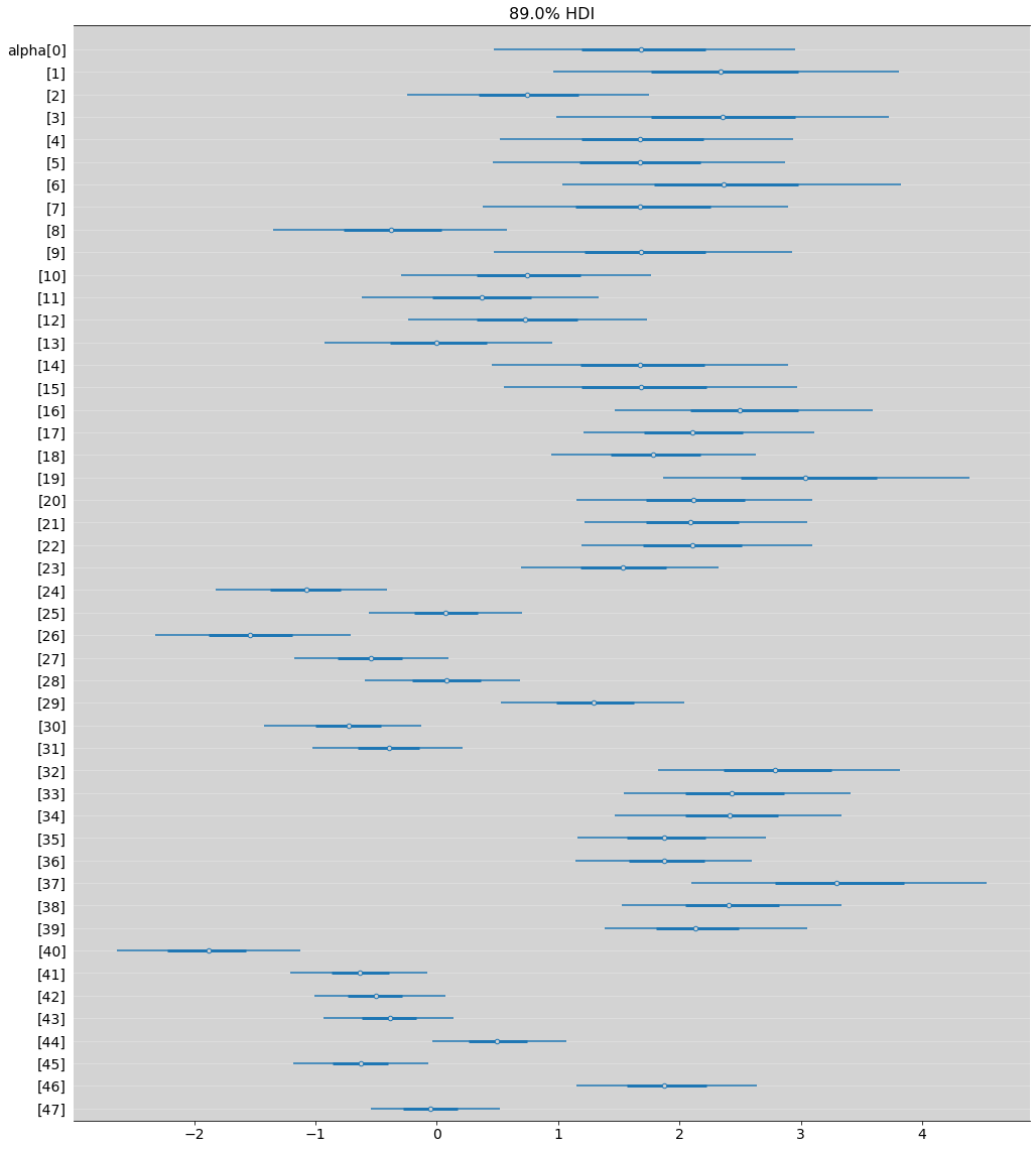
az.plot_forest(model_13_1, hdi_prob=0.89, combined=True, figsize=(17, 20))

plt.grid(axis='y', c='white', alpha=0.3)
plt.show()

R Code 13.3¶

Multilevel model Tadpole¶

\[ S_i \sim Binomial(N_i, p_i) \]

\[ logit(p_i) = \alpha_{TANK[i]} \]

\[ \alpha[j] \sim Normal(\bar{\alpha}, \sigma) \mbox{ - [Adaptative prior]} \]

\[ \bar{\alpha} \sim Normal(0, 1.5) \mbox{ - [prior to average tank]} \]

\[ \sigma \sim Exponential(1) \mbox{ - [prior for standard deviation of tanks]} \]

model = """
    data {
        int qty;
        array[qty] int N;
        array[qty] int survival;
        array[qty] int tank;
    }
    
    parameters {
        vector[qty] alpha;
        real bar_alpha;
        real<lower=0> sigma;
    }
    
    model {
        vector[qty] p;
        
        alpha ~ normal(bar_alpha, sigma);
        
        bar_alpha ~ normal(0, 1.5);
        sigma ~ exponential(1);
        
        for (i in 1:qty){
            p[i] = alpha[ tank[i] ];
            p[i] = inv_logit(p[i]);
        }
    
        survival ~ binomial(N, p);
    }
"""


dat_list = {
    'qty': len(df),
    'tank': df['tank'].to_list(),
    'survival': df['surv'].to_list(),
    'N': df['density'].to_list()
}


posteriori = stan.build(model, data=dat_list)
samples = posteriori.sample(num_chains=4, num_samples=1000)

model_13_2 = az.from_pystan(
    posterior=samples,
    posterior_model=posteriori,
    observed_data=dat_list.keys(),
)

az.summary(model_13_2, hdi_prob=0.89)

	mean	sd	hdi_5.5%	hdi_94.5%	mcse_mean	mcse_sd	ess_bulk	ess_tail	r_hat
alpha[0]	2.120	0.878	0.638	3.364	0.013	0.011	5103.0	2774.0	1.0
alpha[1]	3.042	1.090	1.234	4.649	0.017	0.013	4432.0	3020.0	1.0
alpha[2]	1.012	0.678	-0.009	2.145	0.009	0.008	5420.0	2781.0	1.0
alpha[3]	3.067	1.134	1.212	4.680	0.020	0.017	3701.0	2066.0	1.0
alpha[4]	2.143	0.887	0.787	3.555	0.013	0.011	5244.0	2510.0	1.0
alpha[5]	2.122	0.864	0.782	3.457	0.012	0.010	5285.0	2885.0	1.0
alpha[6]	3.076	1.122	1.159	4.666	0.017	0.014	5095.0	2384.0	1.0
alpha[7]	2.134	0.871	0.681	3.370	0.013	0.010	4979.0	2943.0	1.0
alpha[8]	-0.176	0.624	-1.097	0.884	0.009	0.010	4791.0	2630.0	1.0
alpha[9]	2.131	0.856	0.870	3.516	0.012	0.010	5257.0	2688.0	1.0
alpha[10]	1.009	0.657	-0.059	2.031	0.009	0.008	5011.0	2379.0	1.0
alpha[11]	0.578	0.643	-0.410	1.625	0.009	0.008	5160.0	3014.0	1.0
alpha[12]	1.002	0.643	0.018	2.031	0.009	0.007	5615.0	3058.0	1.0
alpha[13]	0.205	0.619	-0.818	1.132	0.008	0.010	5383.0	2795.0	1.0
alpha[14]	2.144	0.850	0.811	3.456	0.013	0.011	4588.0	2692.0	1.0
alpha[15]	2.130	0.888	0.742	3.503	0.013	0.011	5481.0	2815.0	1.0
alpha[16]	2.930	0.808	1.772	4.282	0.012	0.009	5486.0	2837.0	1.0
alpha[17]	2.414	0.673	1.351	3.467	0.010	0.008	4980.0	2624.0	1.0
alpha[18]	2.029	0.596	1.078	2.965	0.010	0.008	3769.0	2496.0	1.0
alpha[19]	3.668	0.998	2.060	5.129	0.015	0.012	4742.0	2956.0	1.0
alpha[20]	2.401	0.696	1.294	3.475	0.010	0.008	5393.0	2721.0	1.0
alpha[21]	2.400	0.652	1.354	3.378	0.010	0.008	4742.0	2220.0	1.0
alpha[22]	2.402	0.657	1.379	3.436	0.011	0.008	4170.0	2524.0	1.0
alpha[23]	1.705	0.540	0.862	2.557	0.008	0.006	4555.0	2817.0	1.0
alpha[24]	-0.999	0.449	-1.655	-0.244	0.006	0.005	5423.0	2412.0	1.0
alpha[25]	0.163	0.400	-0.491	0.800	0.005	0.006	5549.0	2698.0	1.0
alpha[26]	-1.429	0.503	-2.269	-0.687	0.008	0.006	4286.0	2894.0	1.0
alpha[27]	-0.483	0.410	-1.148	0.160	0.006	0.005	5325.0	3363.0	1.0
alpha[28]	0.157	0.388	-0.489	0.743	0.006	0.005	4797.0	2966.0	1.0
alpha[29]	1.438	0.479	0.657	2.166	0.006	0.005	5631.0	3250.0	1.0
alpha[30]	-0.637	0.412	-1.259	0.053	0.006	0.005	5600.0	2739.0	1.0
alpha[31]	-0.317	0.395	-1.002	0.256	0.006	0.006	5105.0	2842.0	1.0
alpha[32]	3.188	0.771	1.963	4.334	0.012	0.009	4968.0	2644.0	1.0
alpha[33]	2.714	0.639	1.685	3.693	0.009	0.007	4885.0	3002.0	1.0
alpha[34]	2.715	0.657	1.705	3.773	0.010	0.008	4591.0	2027.0	1.0
alpha[35]	2.072	0.519	1.255	2.887	0.008	0.006	4743.0	2557.0	1.0
alpha[36]	2.061	0.514	1.291	2.909	0.008	0.006	4889.0	2645.0	1.0
alpha[37]	3.893	0.955	2.436	5.387	0.015	0.012	4467.0	2872.0	1.0
alpha[38]	2.702	0.641	1.767	3.752	0.010	0.008	4560.0	2247.0	1.0
alpha[39]	2.354	0.562	1.433	3.187	0.009	0.007	4042.0	2801.0	1.0
alpha[40]	-1.799	0.474	-2.528	-1.032	0.007	0.005	4750.0	2938.0	1.0
alpha[41]	-0.573	0.355	-1.133	-0.006	0.005	0.004	4697.0	2564.0	1.0
alpha[42]	-0.456	0.345	-1.001	0.096	0.005	0.004	5231.0	3157.0	1.0
alpha[43]	-0.334	0.343	-0.872	0.226	0.005	0.004	4927.0	3032.0	1.0
alpha[44]	0.582	0.345	0.041	1.143	0.005	0.004	4770.0	3146.0	1.0
alpha[45]	-0.573	0.366	-1.163	0.008	0.005	0.004	5334.0	3158.0	1.0
alpha[46]	2.069	0.522	1.285	2.919	0.008	0.006	4822.0	2614.0	1.0
alpha[47]	-0.000	0.340	-0.524	0.552	0.005	0.006	5063.0	2720.0	1.0
bar_alpha	1.346	0.260	0.940	1.758	0.005	0.003	3131.0	2923.0	1.0
sigma	1.618	0.216	1.263	1.940	0.004	0.003	2491.0	3083.0	1.0

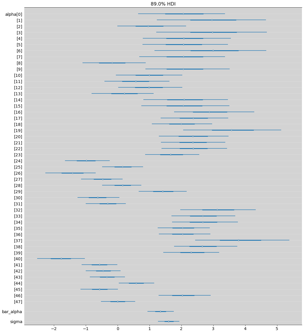
az.plot_forest(model_13_2, hdi_prob=0.89, combined=True, figsize=(17, 20))

plt.grid(axis='y', color='white', alpha=0.3)
plt.show()

R Code 13.4¶

# az.compare(model_13_1, model_13_2)

R Code 13.5¶

means = [ model_13_2.posterior.alpha.sel(alpha_dim_0=(i-1)).values.flatten().mean() for i in df.tank ]
means = inv_logit(means)

# My test, this is not originaly in book
means_13_1 = [ model_13_1.posterior.alpha.sel(alpha_dim_0=(i-1)).values.flatten().mean() for i in df.tank ]
means_13_1 = inv_logit(means_13_1)

bar_alpha_log = model_13_2.posterior.bar_alpha.values.flatten()
bar_alpha = inv_logit(bar_alpha_log)
bar_alpha_mean = bar_alpha.mean() 

sigma_log = model_13_2.posterior.sigma.values.flatten()
sigma = inv_logit(sigma_log)
sigma_mean = sigma.mean()

plt.figure(figsize=(17, 6))
plt.ylim = ([0, 1])

plt.scatter(df.tank, means, edgecolors='black', c='lightgray', s=100)
plt.scatter(df.tank, means_13_1, edgecolors='yellow', c='lightgray', s=100, alpha=0.4)
plt.scatter(df.tank, df.propsurv, c='blue')


plt.axvline(x=15.5, ls='--', color='white', alpha=0.3)
plt.axvline(x=31.5, ls='--', color='white', alpha=0.3)

plt.axhline(y=bar_alpha_mean, ls='--', c='black', alpha=0.7)

plt.text(4, 0.05, 'Small Tank', size=12)
plt.text(22, 0.05, 'Medium Tank', size=12)
plt.text(40, 0.05, 'Large Tank', size=12)

plt.gca().set_ylim(0.0, 1.05)

plt.title('Tadpole survival Tanks')
plt.xlabel('Tank Index')
plt.ylabel('Porportion Survival')

plt.show()

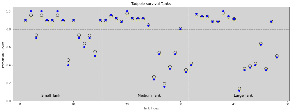
Blue dot: Proportion survival s_i/N_i
Black circle: Multilevel model estimative
Light Yellow: No-pooling estimative

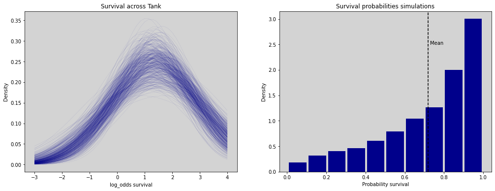
R Code 13.6¶

fig = plt.figure(figsize=(17, 6))
gs = GridSpec(1, 2)

x = np.linspace(-3, 4)

s_sampled = 500

ax1 = fig.add_subplot(gs[0, 0])
log_odds_survival = []
log_odds_sampled_index = np.random.choice(len(bar_alpha_log) ,size=s_sampled, replace=False)

for i in log_odds_sampled_index:
    log_odds_survival.append(stats.norm.pdf(x, bar_alpha_log[i], sigma_log[i]))

for i in range(s_sampled):
    ax1.plot(x, log_odds_survival[i], c='darkblue', linewidth=0.05)
ax1.set_title('Survival across Tank')
ax1.set_xlabel('log_odds survival')
ax1.set_ylabel('Density')
    

ax2 = fig.add_subplot(gs[0, 1])
samples_log = np.random.normal(bar_alpha_log, sigma_log)
ax2.hist(inv_logit(samples_log), rwidth=0.9, color='darkblue', density=True)
ax2.axvline(x=np.mean(inv_logit(samples_log)), c='black', ls='--')
ax2.text(np.mean(inv_logit(samples_log))+0.01, 2.5, 'Mean')

ax2.set_title('Survival probabilities simulations')
ax2.set_xlabel('Probability survival')
ax2.set_ylabel('Density')

plt.show()

13.2 Varing effects and underfitting/overfitting trade-off¶

The model

\[ S_i \sim Binomial(N_i, p_i) \]

\[ logit(p_i) = \alpha_{POND[i]} \]

\[ \alpha_j \sim Normal(\bar{\alpha}, \sigma) \]

\[ \bar{\alpha} \sim Normal(0, 1.5) \]

\[ \sigma \sim Exponential(1) \]

$\bar{\alpha} := $ the avegare log-oods fo survival in the entire population of ponds

$\sigma := $ the standard deviation of the distribution of log-oods of survivial among ponds

$\alpha := $ a vector of individual pond intercepts, one for each pond

R Code 13.7¶

a_bar = 1.5
sigma = 1.5
nponds = 60

repeats = 15

Ni = np.repeat([5, 10, 25, 35], repeats=repeats)

R Code 13.8¶

a_pond = np.random.normal(loc=a_bar, scale=sigma, size=nponds)

R Code 13.9¶

d = {
    'pond': np.arange(nponds) + 1,
    'Ni':Ni,
    'true_a': a_pond,
}

dsim = pd.DataFrame(data=d)
dsim.head()

	pond	Ni	true_a
0	1	5	1.812547
1	2	5	0.484266
2	3	5	2.273773
3	4	5	1.495332
4	5	5	1.674099

R Code 13.10¶

# Code in R -> integer vs numeric

R Code 13.11¶

dsim['Si'] = np.random.binomial(n=dsim['Ni'], p=inv_logit(dsim['true_a']))
dsim.head()

	pond	Ni	true_a	Si
0	1	5	1.812547	5
1	2	5	0.484266	4
2	3	5	2.273773	3
3	4	5	1.495332	3
4	5	5	1.674099	5

R Code 13.12¶

13.2.4 Compute the no-pooling estimates¶

dsim['p_nopool'] = dsim['Si'] / dsim['Ni']
dsim.head()

	pond	Ni	true_a	Si	p_nopool
0	1	5	1.812547	5	1.0
1	2	5	0.484266	4	0.8
2	3	5	2.273773	3	0.6
3	4	5	1.495332	3	0.6
4	5	5	1.674099	5	1.0

R Code 13.13¶

13.2.5 Compute the partial-pooling estimates¶

model = """
    data {
        int N;
        array[N] int pond;  // Pond index
        array[N] int Ni;  // Population in pond[i]
        array[N] int Si;  // Survivals from Ni pond
    }
    
    parameters {
        vector[N] alpha;
        real bar_alpha;
        real<lower=0> sigma;
    }
    
    model {
        vector[N] pi;
        
        // Link
            for (i in 1:N) {
                pi[i] = alpha[ pond[i] ];
                pi[i] = inv_logit(pi[i]);
            }
        
        // Prior
        alpha ~ normal(bar_alpha, sigma);
        
        // Hyper Prior
        bar_alpha ~ normal(0, 1.5);
        sigma ~ exponential(1);
    
        // Likelihood
        Si ~ binomial(Ni, pi);
    }
"""


dat_list = {
    'N': len(dsim),
    'Ni': dsim['Ni'].to_list(),
    'pond': dsim['pond'].to_list(),
    'Si': dsim['Si'].to_list(),
}

posteriori = stan.build(model, data=dat_list)
samples = posteriori.sample(num_chains=4, num_samples=1000)

R Code 13.14¶

model_13_3 = az.from_pystan(
    posterior=samples,
    posterior_model=posteriori,
    observed_data=dat_list
)

az.summary(model_13_3, hdi_prob=0.89)

	mean	sd	hdi_5.5%	hdi_94.5%	mcse_mean	mcse_sd	ess_bulk	ess_tail	r_hat
alpha[0]	2.787	1.241	0.919	4.799	0.019	0.016	4867.0	2442.0	1.0
alpha[1]	1.562	0.969	-0.034	3.021	0.014	0.012	5222.0	2609.0	1.0
alpha[2]	0.721	0.865	-0.728	2.038	0.012	0.012	5554.0	2651.0	1.0
alpha[3]	0.728	0.854	-0.587	2.118	0.013	0.012	4619.0	2732.0	1.0
alpha[4]	2.759	1.252	0.761	4.686	0.019	0.015	4595.0	2736.0	1.0
...	...	...	...	...	...	...	...	...	...
alpha[57]	4.017	1.033	2.446	5.569	0.017	0.014	4304.0	2100.0	1.0
alpha[58]	1.430	0.410	0.782	2.105	0.006	0.004	5454.0	3090.0	1.0
alpha[59]	1.115	0.384	0.451	1.690	0.005	0.004	5327.0	3270.0	1.0
bar_alpha	1.442	0.254	1.026	1.835	0.004	0.003	3741.0	2961.0	1.0
sigma	1.700	0.236	1.320	2.046	0.006	0.004	1522.0	2025.0	1.0

62 rows × 9 columns

R Code 13.15¶

dsim['p_partpool'] = [inv_logit(model_13_3.posterior.alpha.sel(alpha_dim_0=i).values.mean()) for i in range(len(dsim))]
dsim.head()

	pond	Ni	true_a	Si	p_nopool	p_partpool
0	1	5	1.812547	5	1.0	0.941987
1	2	5	0.484266	4	0.8	0.826685
2	3	5	2.273773	3	0.6	0.672823
3	4	5	1.495332	3	0.6	0.674364
4	5	5	1.674099	5	1.0	0.940440

R Code 13.16¶

dsim['p_true'] = inv_logit(dsim['true_a'])
dsim.head()

	pond	Ni	true_a	Si	p_nopool	p_partpool	p_true
0	1	5	1.812547	5	1.0	0.941987	0.859669
1	2	5	0.484266	4	0.8	0.826685	0.618755
2	3	5	2.273773	3	0.6	0.672823	0.906681
3	4	5	1.495332	3	0.6	0.674364	0.816877
4	5	5	1.674099	5	1.0	0.940440	0.842122

R Code 13.17¶

no_pool_error = np.abs(dsim['p_nopool'] - dsim['p_true'])
partpool_error = np.abs(dsim['p_partpool'] - dsim['p_true'])

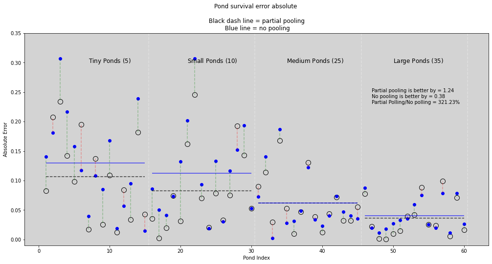
R Code 13.18¶

plt.figure(figsize=(17, 8))
plt.ylim = ([0, 1])
max_lim_graph = 0.3

plt.scatter(dsim.pond, partpool_error, edgecolors='black', c='lightgray', s=100)
plt.scatter(dsim.pond, no_pool_error, c='blue')

qty_unique_ponds = len(dsim['Ni'].unique())
qty_each_ponds = repeats  # The number of repetitions for each element in each pond.


# Vertical lines
for i in range(qty_unique_ponds):
    plt.axvline(x=qty_each_ponds*(i+1) + 0.5, ls='--', color='white', alpha=0.3)
    
    partpool_error_mean = np.mean(partpool_error[(qty_each_ponds*i):(qty_each_ponds*(i+1))])
    no_pool_error_mean = np.mean(no_pool_error[(qty_each_ponds*i):(qty_each_ponds*(i+1))])
    
    plt.hlines(y=partpool_error_mean, xmin=1+(qty_each_ponds*i), xmax=qty_each_ponds+(qty_each_ponds*i), ls='--', colors='black', alpha=0.7)
    plt.hlines(y=no_pool_error_mean, xmin=1+(qty_each_ponds*i), xmax=qty_each_ponds+(qty_each_ponds*i), ls='-', colors='blue', alpha=0.7)

score_no_pooling = 0
score_partial_pooling = 0
    
for i in dsim.pond:
    if no_pool_error[i-1] >= partpool_error[i-1]:  # partial polling is better
        plt.vlines(x=i, ymin=no_pool_error[i-1], ymax=partpool_error[i-1], ls='--', colors='green', alpha=0.3)
        score_partial_pooling += no_pool_error[i-1] - partpool_error[i-1]  # How partial pooling is better
        
    else:  # no pooling is better
        plt.vlines(x=i, ymin=no_pool_error[i-1], ymax=partpool_error[i-1], ls='--', colors='red', alpha=0.3)
        score_no_pooling += partpool_error[i-1] - no_pool_error[i-1]  # How no pooling is better

plt.text(7, max_lim_graph, 'Tiny Ponds ($5$)', size=12)
plt.text(21, max_lim_graph, 'Small Ponds ($10$)', size=12)
plt.text(35, max_lim_graph, 'Medium Ponds ($25$)', size=12)
plt.text(50, max_lim_graph, 'Large Ponds ($35$)', size=12)

plt.text(47, 0.25, f'Partial pooling is better by = {round(score_partial_pooling, 2)}')
plt.text(47, 0.24, f'No pooling is better by = {round(score_no_pooling, 2)}')
plt.text(47, 0.23, f'Partial Polling/No polling = {round((score_partial_pooling/score_no_pooling)*100, 2)}%')


plt.gca().set_ylim(-0.01, max_lim_graph + 0.05)

plt.title('Pond survival error absolute \n\n Black dash line = partial pooling \n Blue line = no pooling')
plt.xlabel('Pond Index')
plt.ylabel('Absolute Error')

plt.show()

R Code 13.20¶

# Reuse code in using Rethinking packages in R, here is automatically reuse!
# Just re-run from R Code 13.7

13.3 More than one type of cluster¶

Multilevel Chimpanzees¶

\[ L_i \sim Binomial(1, p_i) \]

\[ logit(p_i) = \alpha_{ACTOR[i]} + \gamma_{BLOCK[i]} + \beta_{TREATMENT[i]} \]

\[ \beta_j \sim Normal(0, 0.5) \mbox{ , } j \in \{1, ... ,4\} \]

\[ \alpha_j \sim Normal(\bar{\alpha}, \sigma_\alpha) \mbox{ , } j \in \{1, ... ,7\} \]

\[ \gamma_j \sim Normal(0, \sigma_\gamma) \mbox{ , } j \in \{1, ... ,6\} \]

\[ \bar{\alpha} \sim Normal(0, 1.5) \]

\[ \sigma_{\alpha} \sim Exponential(1) \]

\[ \sigma_{\gamma} \sim Exponential(1) \]

R Code 13.21¶

# Previous chimpanzees models is in chapter 11

df = pd.read_csv('./data/chimpanzees.csv', sep=';')
df.head()

	actor	recipient	block	trial	prosoc_left	chose_prosoc	pulled_left
0	1	NaN	1	2	0	1	0
1	1	NaN	1	4	0	0	1
2	1	NaN	1	6	1	0	0
3	1	NaN	1	8	0	1	0
4	1	NaN	1	10	1	1	1

df['treatment'] = 1 + df['prosoc_left'] + 2 * df['condition']
df.head()

	actor	recipient	block	trial	prosoc_left	chose_prosoc	pulled_left	treatment
0	1	NaN	1	2	0	1	0	1
1	1	NaN	1	4	0	0	1	1
2	1	NaN	1	6	1	0	0	2
3	1	NaN	1	8	0	1	0	1
4	1	NaN	1	10	1	1	1	2

model = """
    data {
        int N;
        int qty_chimpanzees;
        int qty_blocks;
        int qty_treatments;
        
        array[N] int pulled_left;
        array[N] int actor;
        array[N] int block;
        array[N] int treatment;
    }
    
    parameters {
        vector[qty_treatments] beta;
        
        vector[qty_chimpanzees] alpha;
        real bar_alpha;
        real<lower=0> sigma_alpha;
        
        vector[qty_blocks] gamma;
        real<lower=0>  sigma_gamma;
           
    }
    
    model {
        vector[N] p;
    
        // priors
        beta ~ normal(0, 0.5);
        
        alpha ~ normal(bar_alpha, sigma_alpha);
        bar_alpha ~ normal(0, 1.5);
        sigma_alpha ~ exponential(1);
        
        gamma ~ normal(0, sigma_gamma);
        sigma_gamma ~ exponential(1);
        
        // link
        for (i in 1:N){
            p[i] = alpha[ actor[i] ] + gamma[ block[i] ] + beta[ treatment[i] ];
            p[i] = inv_logit(p[i]);
        }
        
        // linkelihood
        pulled_left ~ binomial(1, p);
    }

"""

dat_list = df[['pulled_left', 'actor', 'block', 'treatment']].to_dict('list')
dat_list['N'] = len(df)
dat_list['qty_chimpanzees'] = len(df['actor'].unique())
dat_list['qty_blocks'] = len(df['block'].unique())
dat_list['qty_treatments'] = len(df['treatment'].unique())

posteriori = stan.build(model, data=dat_list)
samples = posteriori.sample(num_chains=4, num_samples=1000)

R Code 13.22¶

model_13_4 = az.from_pystan(
    posterior=samples,
    posterior_model=posteriori,
    observed_data=dat_list
)

az.summary(model_13_4, hdi_prob=0.89)

	mean	sd	hdi_5.5%	hdi_94.5%	mcse_mean	mcse_sd	ess_bulk	ess_tail	r_hat
beta[0]	-0.178	0.296	-0.569	0.352	0.042	0.030	54.0	1029.0	1.06
beta[1]	0.332	0.321	-0.083	0.828	0.077	0.056	20.0	1608.0	1.14
beta[2]	-0.537	0.308	-0.994	-0.069	0.059	0.043	31.0	1329.0	1.09
beta[3]	0.232	0.297	-0.221	0.702	0.046	0.033	45.0	1159.0	1.06
alpha[0]	-0.263	0.405	-0.829	0.320	0.106	0.077	17.0	1605.0	1.17
alpha[1]	4.763	1.249	2.811	6.460	0.035	0.025	1182.0	1293.0	1.03
alpha[2]	-0.624	0.347	-1.205	-0.104	0.021	0.024	400.0	1396.0	1.03
alpha[3]	-0.588	0.393	-1.237	-0.112	0.085	0.061	24.0	1595.0	1.12
alpha[4]	-0.275	0.387	-0.899	0.220	0.092	0.066	20.0	860.0	1.14
alpha[5]	0.620	0.353	0.033	1.161	0.016	0.011	507.0	1421.0	1.03
alpha[6]	2.121	0.437	1.383	2.782	0.013	0.009	1137.0	1182.0	1.26
bar_alpha	0.678	0.714	-0.443	1.795	0.089	0.063	65.0	1892.0	1.04
sigma_alpha	2.069	0.624	1.058	2.831	0.036	0.026	135.0	1582.0	1.04
gamma[0]	-0.154	0.208	-0.471	0.101	0.025	0.018	76.0	1477.0	1.04
gamma[1]	0.038	0.167	-0.227	0.299	0.004	0.006	2537.0	1366.0	1.27
gamma[2]	0.043	0.173	-0.214	0.319	0.004	0.006	1370.0	1513.0	1.05
gamma[3]	0.005	0.164	-0.272	0.248	0.003	0.005	2437.0	1654.0	1.29
gamma[4]	-0.030	0.172	-0.286	0.246	0.003	0.005	2766.0	1883.0	1.28
gamma[5]	0.103	0.187	-0.160	0.402	0.014	0.010	395.0	1375.0	1.04
sigma_gamma	0.196	0.173	0.017	0.405	0.034	0.025	11.0	4.0	1.29

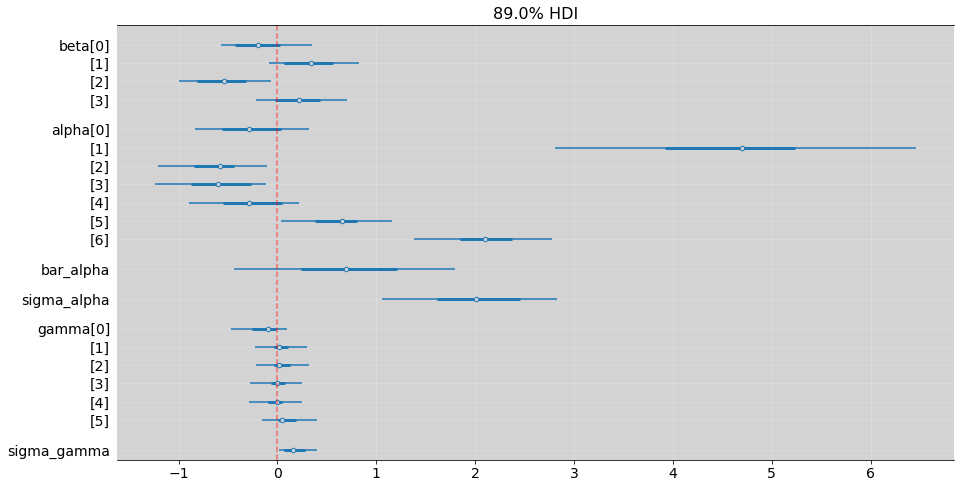
az.plot_forest(model_13_4, hdi_prob=0.89, combined=True, figsize=(15, 8))
plt.grid('--', color='white', alpha=0.2)
plt.axvline(x=0, color='red', alpha=0.5, ls='--')
plt.show()

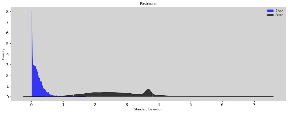
plt.figure(figsize=(17, 6))

az.plot_dist(
    [model_13_4.posterior.sigma_gamma], color='blue', quantiles=[.05, .89]
)

az.plot_dist(
    [model_13_4.posterior.bar_alpha + model_13_4.posterior.sigma_alpha],
    color='black', quantiles=[.05, .89]
)

plt.legend(['Block', 'Actor'])
plt.title('Posteioris')
plt.ylabel('Density')
plt.xlabel('Standard Deviation')
plt.show()

R Code 13.23¶

model = """
    data {
        int N;
        int qty_chimpanzees;
        int qty_blocks;
        int qty_treatments;
        
        array[N] int pulled_left;
        array[N] int actor;
        array[N] int block;
        array[N] int treatment;
    }
    
    parameters {
        vector[qty_treatments] beta;
        
        vector[qty_chimpanzees] alpha;
        real bar_alpha;
        real<lower=0> sigma_alpha;   
    }
    
    model {
        vector[N] p;
    
        // priors
        beta ~ normal(0, 0.5);
        
        alpha ~ normal(bar_alpha, sigma_alpha);
        bar_alpha ~ normal(0, 1.5);
        sigma_alpha ~ exponential(1);
        
        // link
        for (i in 1:N){
            p[i] = alpha[ actor[i] ] + beta[ treatment[i] ];
            p[i] = inv_logit(p[i]);
        }
        
        // linkelihood
        pulled_left ~ binomial(1, p);
    }

"""

dat_list = df[['pulled_left', 'actor', 'block', 'treatment']].to_dict('list')
dat_list['N'] = len(df)
dat_list['qty_chimpanzees'] = len(df['actor'].unique())
dat_list['qty_blocks'] = len(df['block'].unique())
dat_list['qty_treatments'] = len(df['treatment'].unique())

posteriori = stan.build(model, data=dat_list)
samples = posteriori.sample(num_chains=4, num_samples=1000)

model_13_5 = az.from_pystan(
    posterior=samples,
    posterior_model=posteriori,
    observed_data=dat_list.keys()
)

R Code 13.24¶

# az.compare(model_13_4, model_13_5)

R Code 13.25¶

model = """
    data {
        int N;
        int qty_chimpanzees;
        int qty_blocks;
        int qty_treatments;
        
        array[N] int pulled_left;
        array[N] int actor;
        array[N] int block;
        array[N] int treatment;
    }
    
    parameters {
        vector[qty_treatments] beta;
        real<lower=0>  sigma_beta;

        vector[qty_chimpanzees] alpha;
        real bar_alpha;
        real<lower=0> sigma_alpha;
        
        vector[qty_blocks] gamma;
        real<lower=0>  sigma_gamma;
        
    }
    
    model {
        vector[N] p;
    
        // priors
        beta ~ normal(0, sigma_beta);
        sigma_beta ~ exponential(1);
        
        alpha ~ normal(bar_alpha, sigma_alpha);
        bar_alpha ~ normal(0, 1.5);
        sigma_alpha ~ exponential(1);
        
        gamma ~ normal(0, sigma_gamma);
        sigma_gamma ~ exponential(1);
        
        // link
        for (i in 1:N){
            p[i] = alpha[ actor[i] ] + gamma[ block[i] ] + beta[ treatment[i] ];
            p[i] = inv_logit(p[i]);
        }
        
        // linkelihood
        pulled_left ~ binomial(1, p);
    }

"""

dat_list = df[['pulled_left', 'actor', 'block', 'treatment']].to_dict('list')
dat_list['N'] = len(df)
dat_list['qty_chimpanzees'] = len(df['actor'].unique())
dat_list['qty_blocks'] = len(df['block'].unique())
dat_list['qty_treatments'] = len(df['treatment'].unique())

posteriori = stan.build(model, data=dat_list)
samples = posteriori.sample(num_chains=4, num_samples=1000)

model_13_6 = az.from_pystan(
    posterior=samples,
    posterior_model=posteriori,
    observed_data=dat_list.keys()
)

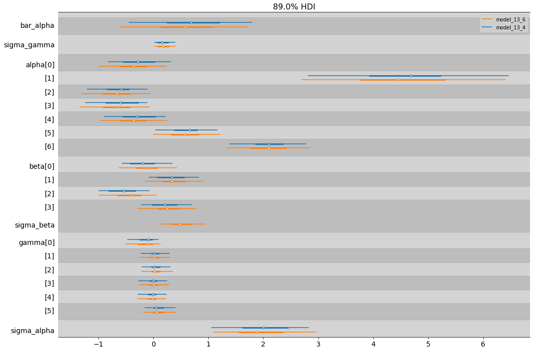
az.plot_forest([model_13_4, model_13_6], combined=True, figsize=(17,12), hdi_prob=0.89,
              model_names = ["model_13_4", "model_13_6"])
plt.show()

13.4 Divergent Transitions and non-centered priors¶

R Code 13.26¶

model = """
    parameters {
        real v;
        real x;
    }
    
    model {
        v ~ normal(0, 3);
        x ~ normal(0, exp(v));
    }
"""

posteriori = stan.build(model)
samples = posteriori.sample(num_chains=4, num_samples=1000)

model_13_5 = az.from_pystan(
    posterior=samples,
    posterior_model=posteriori,
)

az.summary(model_13_5, hdi_prob=0.89)

	mean	sd	hdi_5.5%	hdi_94.5%	mcse_mean	mcse_sd	ess_bulk	ess_tail	r_hat
v	3.515	1.508	1.243	5.486	0.208	0.148	37.0	26.0	1.1
x	-34.371	286.623	-142.353	209.821	20.340	14.404	290.0	232.0	1.1

R Code 13.27¶

model = """
    parameters {
        real v;
        real z;
    }
    
    model {
        v ~ normal(0, 3);
        z ~ normal(0, 1);
    }
    
    generated quantities {
        real x;
        
        x = z*exp(v);
    }
"""

posteriori = stan.build(model)
samples = posteriori.sample(num_chains=4, num_samples=1000)

model_13_6 = az.from_pystan(
    posterior=samples,
    posterior_model=posteriori,
)

az.summary(model_13_6, hdi_prob=0.89)

	mean	sd	hdi_5.5%	hdi_94.5%	mcse_mean	mcse_sd	ess_bulk	ess_tail	r_hat
v	0.055	2.991	-4.401	5.018	0.050	0.048	3573.0	2181.0	1.0
z	0.018	0.998	-1.515	1.663	0.018	0.015	3015.0	2616.0	1.0
x	4.028	3223.155	-22.220	30.356	50.982	36.052	2943.0	2668.0	1.0

13.4.2 Non-centered chimpanzees¶

R Code 13.28¶

# Don't have apapt_delta in pystan3, until today.

R Code 13.29¶

\[ L_i \sim Binomial(1, p_i) \]

\[ logit(p_i) = \bar{\alpha} + z_{ACTOR[i]} \sigma_\alpha + x_{BLOCK[i]}\sigma_\gamma + \beta_{TREATMENT[i]} \]

To Actor: $$ \bar{\alpha} \sim Normal(0, 1.5) $$

\[ z_j \sim Normal(0, 1) \]

\[ \sigma_\alpha \sim Exponential(1) \]

To Block:

\[ x_j \sim Normal(0, 1) \]

\[ \sigma_\gamma \sim Exponential(1) \]

To Treatment:

\[ \beta_j \sim Normal(0, 0.5) \]

Where, each actor is defined by:

\[ \alpha_j = \bar{\alpha} + z_j\sigma_\alpha \]

and, each block is defined by:

\[ \gamma_j = x_j\sigma_\gamma \]

model = """
    data {
        int N;
        int qty_chimpanzees;
        int qty_blocks;
        int qty_treatments;
        
        array[N] int pulled_left;
        array[N] int actor;
        array[N] int block;
        array[N] int treatment;
    }
    
    parameters {
        // To treatments
        vector[qty_treatments] beta;
        
        // To actors
        real bar_alpha;
        vector[qty_chimpanzees] z;
        real<lower=0> sigma_alpha;
        
        // To block
        vector[qty_blocks] x;
        real<lower=0>  sigma_gamma;
    }
    
    model {
        vector[N] p;
    
        // priors
        beta ~ normal(0, 0.5);  // treatment
        z ~ normal(0, 1);  // actor
        x ~ normal(0, 1);  // block 
        
        bar_alpha ~ normal(0, 1.5);  // Intercept to alpha (actor)
        
        sigma_alpha ~ exponential(1);
        sigma_gamma ~ exponential(1);
        
        // Link
        for (i in 1:N){
            p[i] = bar_alpha  + z[ actor[i] ]*sigma_alpha +  x[ block[i] ]*sigma_gamma + beta[ treatment[i] ];
            p[i] = inv_logit(p[i]);
        }
        
        // Linkelihood
        pulled_left ~ binomial(1, p);
    }
    
    generated quantities {
        vector[qty_chimpanzees] alpha;
        vector[qty_blocks] gamma;
        
        alpha = bar_alpha + z*sigma_alpha;
        gamma = x*sigma_gamma;
    }

"""

dat_list = df[['pulled_left', 'actor', 'block', 'treatment']].to_dict('list')
dat_list['N'] = len(df)
dat_list['qty_chimpanzees'] = len(df['actor'].unique())
dat_list['qty_blocks'] = len(df['block'].unique())
dat_list['qty_treatments'] = len(df['treatment'].unique())

posteriori = stan.build(model, data=dat_list)
samples = posteriori.sample(num_chains=4, num_samples=1000)

model_13_4_nc = az.from_pystan(
    posterior=samples,
    posterior_model=posteriori,
    observed_data=dat_list.keys()
)

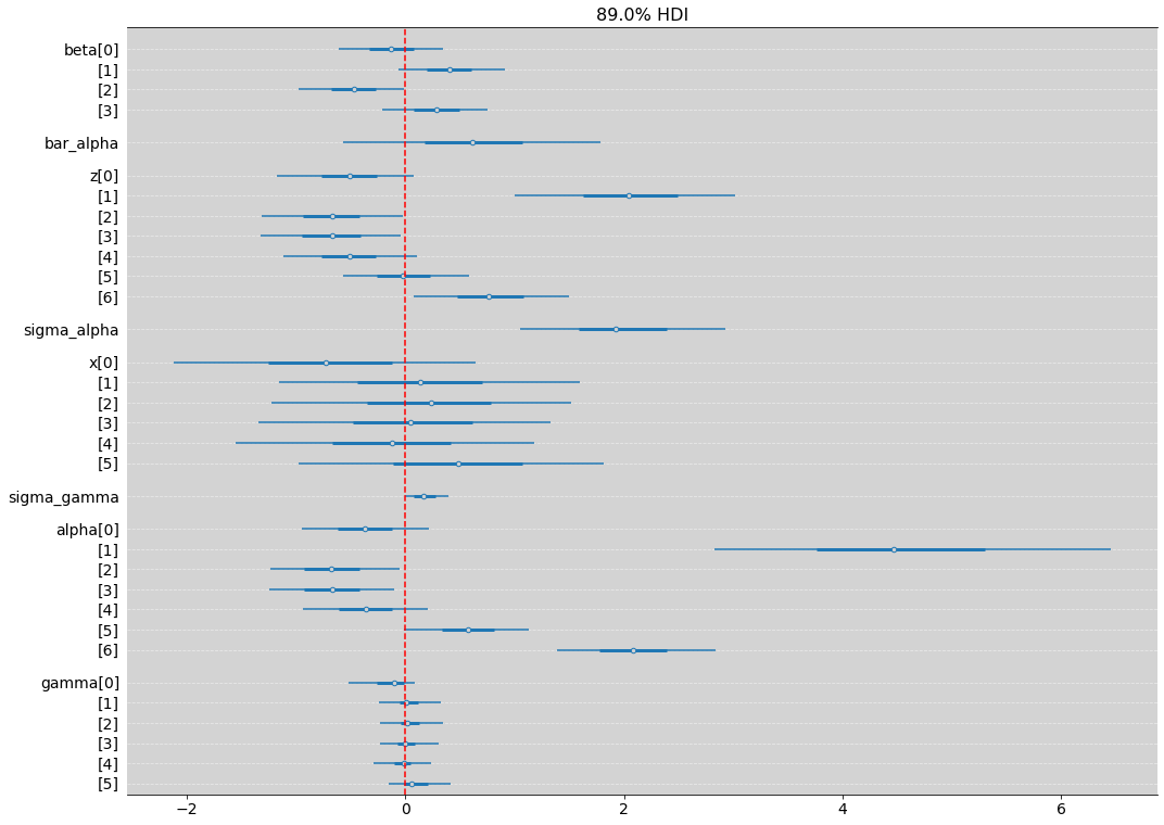
az.plot_forest(model_13_4_nc, hdi_prob=0.89, combined=True, figsize=(17, 13))

plt.axvline(x=0, ls='--', color='red')
plt.grid(axis='y', color='white', ls='--', alpha=0.5)
plt.show()

R Code 13.30¶

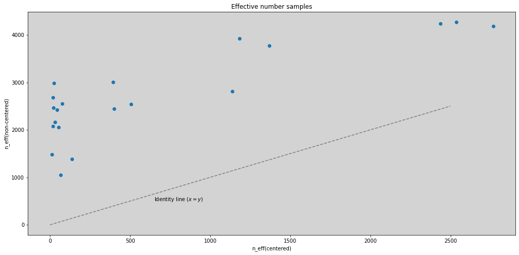
# Extract features from ess

# non-centered
ess_nc = np.array(az.ess(model_13_4_nc, var_names=['alpha']).alpha.values)
ess_nc = np.append(ess_nc, az.ess(model_13_4_nc, var_names=['beta']).beta.values)
ess_nc = np.append(ess_nc, az.ess(model_13_4_nc, var_names=['gamma']).gamma.values)
ess_nc = np.append(ess_nc, az.ess(model_13_4_nc, var_names=['bar_alpha']).bar_alpha.values)
ess_nc = np.append(ess_nc, az.ess(model_13_4_nc, var_names=['sigma_alpha']).sigma_alpha.values)
ess_nc = np.append(ess_nc, az.ess(model_13_4_nc, var_names=['sigma_gamma']).sigma_gamma.values)

# centered
ess_c = np.array(az.ess(model_13_4, var_names=['alpha']).alpha.values)
ess_c = np.append(ess_c, az.ess(model_13_4, var_names=['beta']).beta.values)
ess_c = np.append(ess_c, az.ess(model_13_4, var_names=['gamma']).gamma.values)
ess_c = np.append(ess_c, az.ess(model_13_4, var_names=['bar_alpha']).bar_alpha.values)
ess_c = np.append(ess_c, az.ess(model_13_4, var_names=['sigma_alpha']).sigma_alpha.values)
ess_c = np.append(ess_c, az.ess(model_13_4, var_names=['sigma_gamma']).sigma_gamma.values)

plt.figure(figsize=(17, 8))

plt.scatter(ess_c, ess_nc)

plt.plot([0, 2500], [0, 2500], ls='--', c='k', alpha=0.4)
plt.text(650, 500, 'Identity line ($x=y$)')

plt.title('Effective number samples')
plt.xlabel('n_eff(centered)')
plt.ylabel('n_eff(non-centered)')

plt.show()

	actor	recipient	block	trial	prosoc_left	chose_prosoc	pulled_left	treatment
0	1	NaN	1	2	0	1	0	1
1	1	NaN	1	4	0	0	1	1
2	1	NaN	1	6	1	0	0	2
3	1	NaN	1	8	0	1	0	1
4	1	NaN	1	10	1	1	1	2

	actor	recipient	block	trial	prosoc_left	chose_prosoc	pulled_left	treatment
0	1	NaN	1	2	0	1	0	1
1	1	NaN	1	4	0	0	1	1
2	1	NaN	1	6	1	0	0	2
3	1	NaN	1	8	0	1	0	1
4	1	NaN	1	10	1	1	1	2

Statistical Rethinking

13 - Modelos com Memória¶

Imports, loadings and functions¶

13.1 Example: Multilevel tadpoles¶

R Code 13.1¶

R Code 13.2¶

R Code 13.3¶

Multilevel model Tadpole¶

R Code 13.4¶

R Code 13.5¶

R Code 13.6¶

13.2 Varing effects and underfitting/overfitting trade-off¶

R Code 13.7¶

R Code 13.8¶

R Code 13.9¶

R Code 13.10¶

R Code 13.11¶

R Code 13.12¶

13.2.4 Compute the no-pooling estimates¶

R Code 13.13¶

13.2.5 Compute the partial-pooling estimates¶

R Code 13.14¶

R Code 13.15¶

R Code 13.16¶

R Code 13.17¶

R Code 13.18¶

R Code 13.20¶

13.3 More than one type of cluster¶

Multilevel Chimpanzees¶

R Code 13.21¶

R Code 13.22¶

R Code 13.23¶

R Code 13.24¶

R Code 13.25¶

13.4 Divergent Transitions and non-centered priors¶

R Code 13.26¶

R Code 13.27¶

13.4.2 Non-centered chimpanzees¶

R Code 13.28¶

R Code 13.29¶

R Code 13.30¶

	actor	recipient	block	trial	prosoc_left	chose_prosoc	pulled_left	treatment
0	1	NaN	1	2	0	1	0	1
1	1	NaN	1	4	0	0	1	1
2	1	NaN	1	6	1	0	0	2
3	1	NaN	1	8	0	1	0	1
4	1	NaN	1	10	1	1	1	2